Geodesic Cutoff

**Figure:** Example of an augmented slice from a pair of faces and GMDS applied to these

The core supposition or hypothesis here is that by better selecting boundaries of the surfaces - using geodesic means - the innately geodesic method which is GMDS will perform a lot better and hardly suffer from insufficient information, commonly caused due to Euclidean cropping criteria (as attempted beforehand). For consistency, the experiments that follow will adhere to this 'half face' approach as a given. Realistically, taking a hybrid of features and applying LDA or integrating over them might work better. This is also well supposed by the geodesic masking function. Rather than scoring based on just two surfaces, it is possible to compare subsets of these, with or without fiducial points as a key component to latch the sub-surfaces onto (e.g. eye corners).

Early exploration of our problem revolves around the effect of varying the point around which surfaces get carved. It can be shown that, even for the same person (i.e. same face), the effect of moving that point is as severe as comparing two different faces, so this point is very prone to change the results (a sensitivity-related issue). An interesting experiment might be to distance oneself from this point by controlled and gradually-increasing amounts and then rerun experiments of recognition, seeing how accuracy of this point's allocation affects performance and how much degradation is caused by missing it even very slightly. The location of the features with sub-pixel accuracy cannot be guaranteed, so this might be important to do as a form of sanity check.

Then we have a case of Euclidean plus geodesic cutoff depending on the side, with a fixed point below the eye. The stress/mismatch/distance too is being shown at each point. It helps show the difference, but doing this more properly with geodesic distances all around is probably best. In terms of results, it seems promising, but more elaborate experiments are needed before arriving at any such a conclusion. Using just the nose area for matching has proven to be a poor approach based on some rudimentary tests, but maybe this can be improved shall the need for piece-wise feature-based comparison arise. The geodesic cutoff examples are shown in figures $[*]$ , $[*]$ , $[*]$ , and $[*]$ .

**Figure:** Results of a comparison between arbitrary bits where some boundaries are a Euclidean cutoff and some are geodesic

**Figure:** Results of a comparison between consistently chosen bits (near the eye) where some boundaries are a Euclidean cutoff and some are geodesic

**Figure:** Results of a comparison between surfaces that are mostly carved out of a geodesic boundary

**Figure:** Results of a comparison between noses with a boundary defined by geodesic distance constraints

We shall use the following feature point selection and geodesic circle (support) strategy. If without loss of generality we select the nose and eyes as the features and our geodesic distance ambiguity of the feature selection is $\delta_{a}$ , then for the gallery (target) surface, we define the support as the union of $r+\delta_{a}$ geodesic circles about each feature point ( $\delta_{a}$ and

could be different for each feature). The probe surface should then be defined as the union of radius r-geodesic circles about the features.

This way we try to embed a smaller surface into a larger one, where the larger one is large by the amount of ambiguity of the selected feature (we would like to assume it would be small, but not too small, one would say, 5mm).

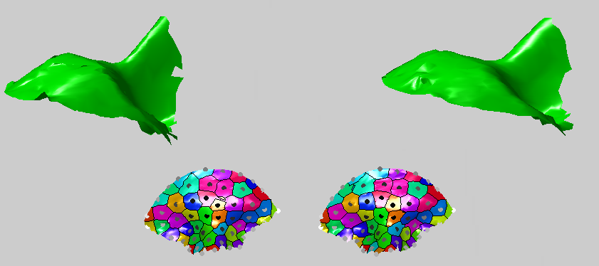
3 points were spread rigidly around the image to mark the centres of points which define geodetically-bounded surfaces. One of these is the tip of the nose. In order to prevent the mouth, for example, from entering the surface (it depends on the length of the nose and its vertical component prevents sufficient point sampling due to the camera's angle), there is a Euclidean concern around there, which explains the flat boundary at the bottom (Figure $[*]$ ). 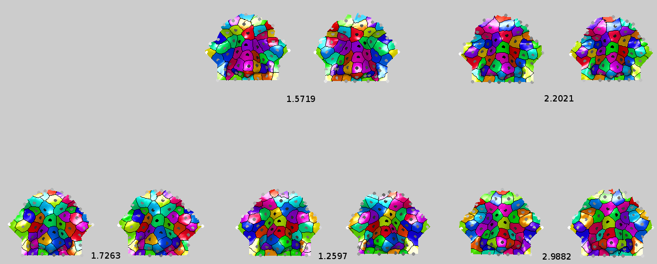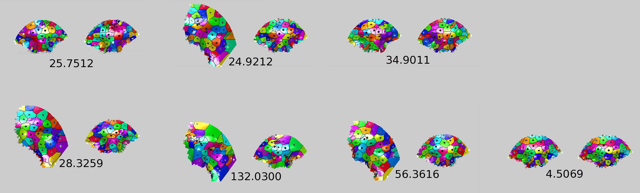The results can be properly explored once a tolerance component is added to the probe or the gallery (consistently for score stability) and another quick set of evaluations was run on a set where the carving was based on the forehead and nose rather than the eyes. (Figure $[*]$ ) There is probably too little information of high entropy around the forehead, though. Sometimes there is hair there.

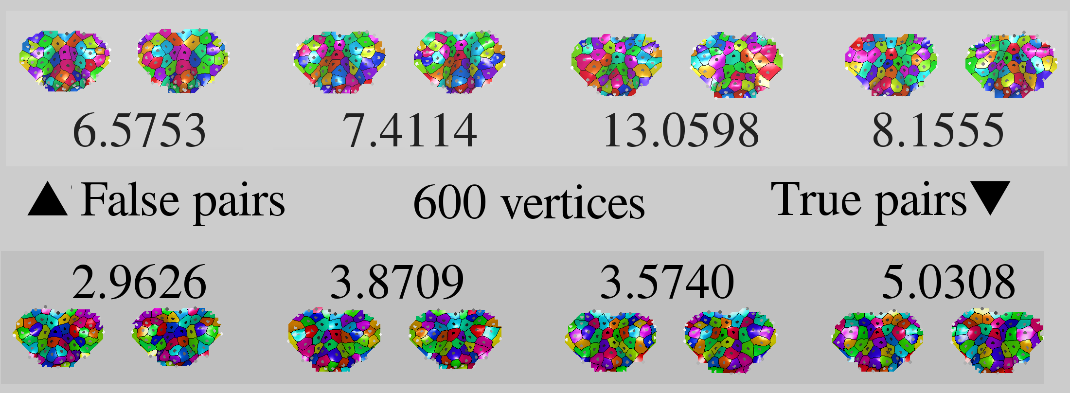
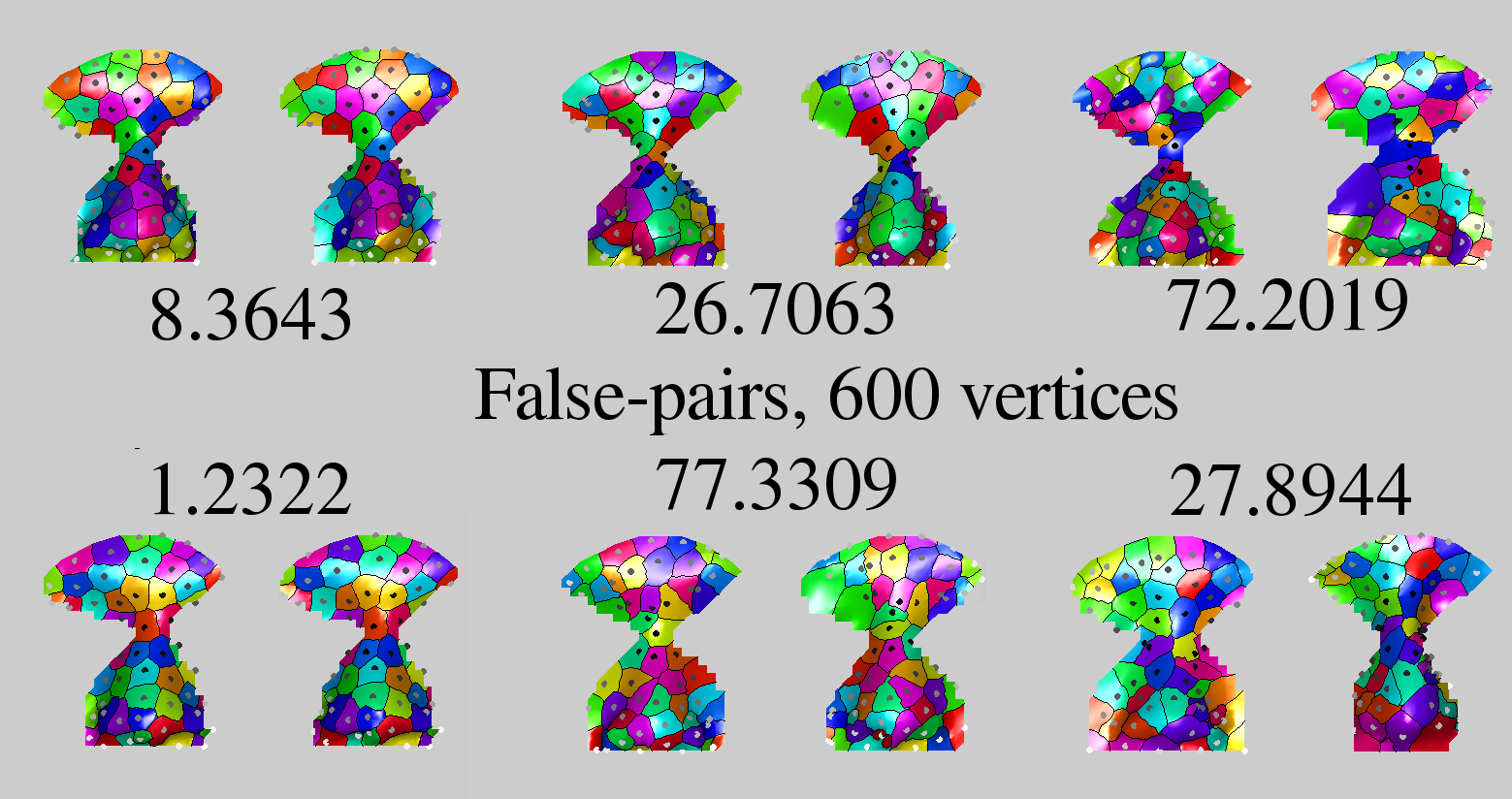
**Figure:** A preliminary look at a predominantly geodesic mask and how it separates pairs from different people (top) and pairs from the same person (bottom)

**Figure:** An experimentation with a mask that includes points around the forehead and around the nose

In terms of performance, with just 600 vertices it does a lot worse than the Euclidean approach with a lot more vertices.

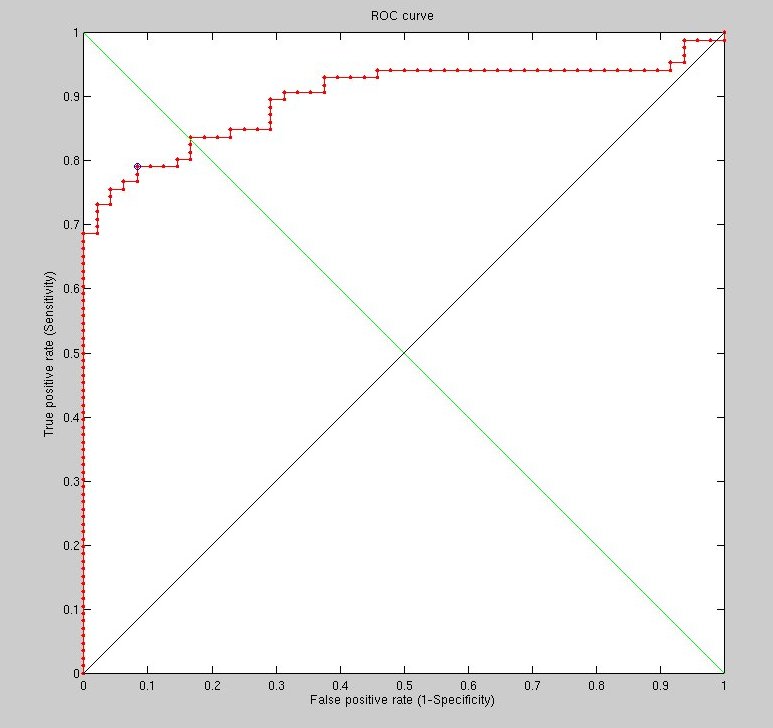
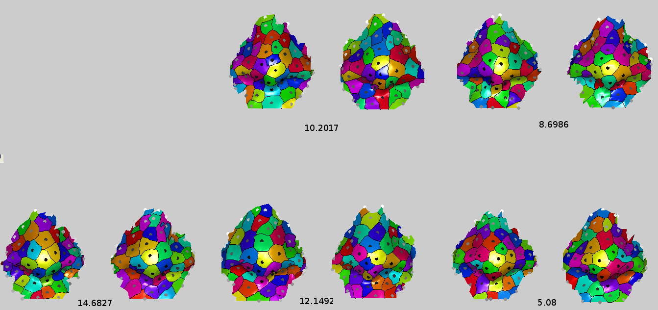
**Figure:** With just 600 vertices, the ROC curve shows unimpressive ability to distinguish between true pairs and false pairs

As we rerun with high density, the results change. Increasing the number of vertices to 2420 improves the results considerably. Some results are shown in Figure u $[*]$ and Figure $[*]$ show some early results.

It is hard to make the case for surface sizes that are not as equal as possible, based on the signal (similarity which is still too noisy). At a coarse and fine levels too, the similarity is not great when geodesic measures are used to carve the surface. By going much higher in terms of resolution we can approach or exceed 95% recognition rate, but to reach 99% or thereabouts there will be further exploration of what needs tweaking, based on pairs where misclassification occurs.

**Figure:** The effect of increasing the number of vertices to 2420.

**Figure:** Improved performance with slight changes in surface size for the gallery

To define much higher resolution, there are several things here and they are all program parameters. First we have raw image signal. Then there is the sampling of the image and also the size of triangles we turn the image into, inversely proportional to their number. The triangulation goes through remeshing and then fed into GMDS, which also can find

correspondences, yielding a matrix smaller than the FMM results. All of these parameters affect speed and some affect stability too. The latest results use 2420 vertices, but the next experiments will look a little at how this can be improved. For instance, changing the geodesic thresholds helps refine the area of consideration. It's unclear how exactly.

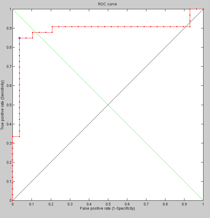
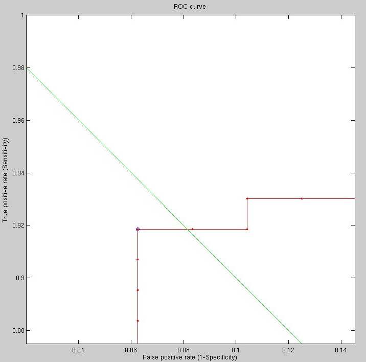
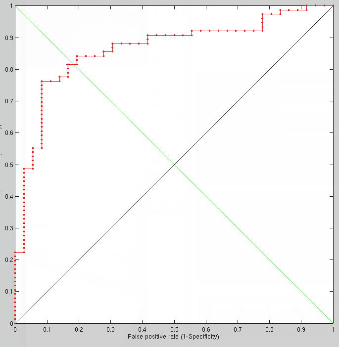
The sampling density is still not so high as it ought to be as this leads to some freezes and other issues (if this is attempted, there are also RAM constraints). However, two additional experiments were run to study the effects of changing the geodesic distances around the eyes and nose (see Figure $[*]$ ). When pushed too far outwards, performance dropped to under 90% recognition rare (Figure $[*]$ ). It is easy to get a 'feel' for what works better and what works poorly based on about 100 test pairs, assessing the results on a comparative basis. Ideally, however, if stability issues can be improved, then the overnight experiments can be run reliably rather than just halt some time over the course of the night.

At the moment, surfaces are being sampled by taking only a separation of 5 pixels between points. In the past that was 2 pixel (range image) and to overcome this loss of signal one can take a local average, which we have not done yet in the experiments. It would make sense to try this.

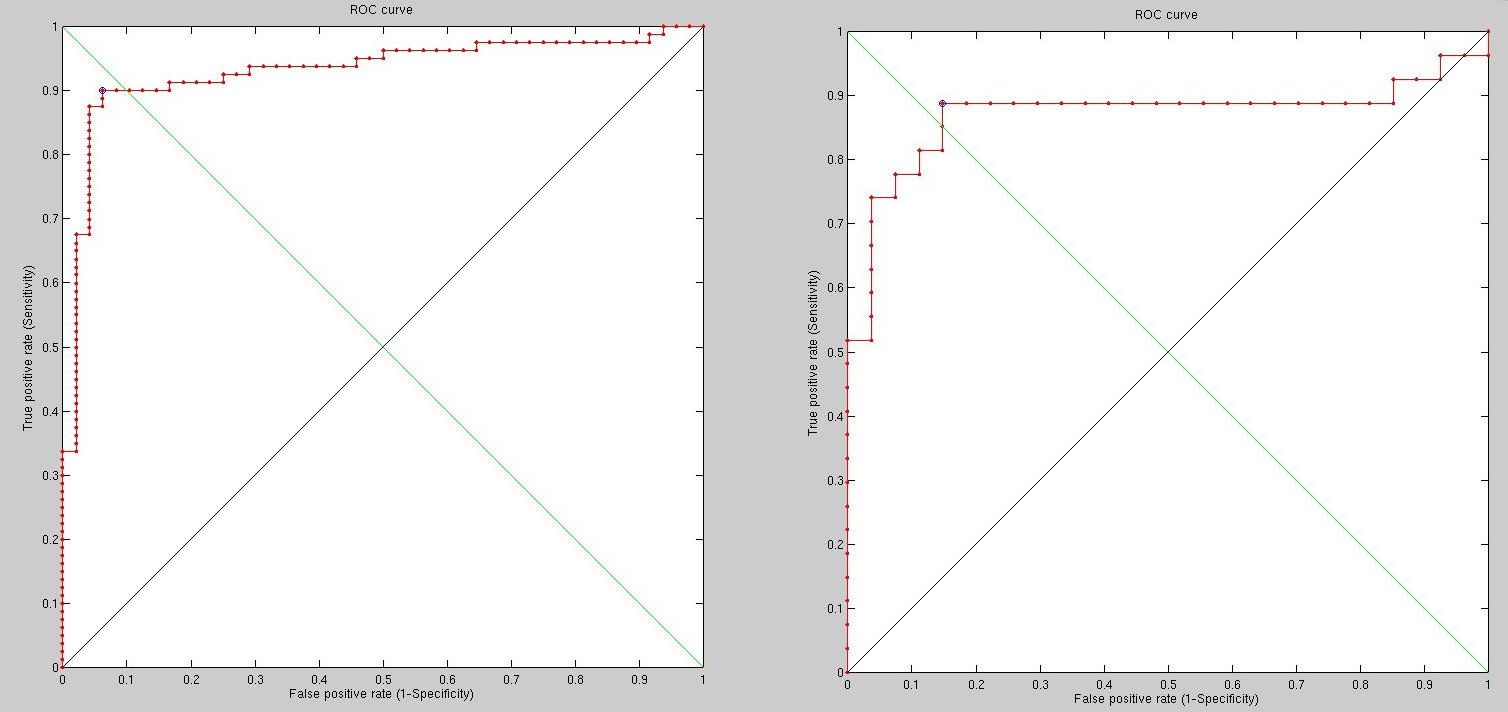
**Figure:** The result of changing the border threshold for surface carving

**Figure:** The result of growing the surface too big

Oddly enough, experiments which test the averaging of range images (for the sake of better sampling before triangulation) actually indicate that the averaging reduces recognition rates (Figure $[*]$ . This performance difference has a direct correlation because all the other conditions remained identical. This seems to concur with previous such experiments - those with PCA. How quaint.

Before scaling everything using PCA (to improve the results) it is probably important to ensure that GMDS is performing as well as possible. Right now there is no spatial scaling applied to the score, notably based on the variability of one area compared to another (e.g. rigidness around the nose, unlike the centre of the eye).

**Figure:** Performance with (left) and without averaging (right) of the arrange image for better sampling of the GMDS process

To re-define the averaging process we apply, what we mean by averaging range images is basically down-sampling the images, or at least the logical equivalent of that.

When the range image is turned into a mesh of triangles there needs to be a discrete sampling of points and the way this is done at the moment involves taking the points within the geodesic mask, then either sub-sampling those (picking with gaps) or talking all of them - about 50,000-60,000 vertices - then remeshing to make things more scalable. The vertices used vary in terms of their number, usually between 600 to 3000 depending on the experiment. It's O(N^2) for FMM, so there need to be reasonable limits. GMDS is sensitive and prone to crashes when the points are picked very densely.

The grid on which you we the

operation has nothing to do with the number of points, i.e. we work with the original resolution of the mesh and pick a small number preferably with farthest point sampling points to embed.

To clarify, there are two phases where FMM is involved. One is the selection of the surfaces on which to perform a comparison. This requires a Fast Marching operation which then helps define what makes the cut and what doesn't. Following that phase we are left with fewer sample points (or fewer triangles) to actually run GMDS on. It is then that GMDS in general (encompassing FMM) depends on the amount of data available to it. What's unclear is, what number of triangles are desirable on each surface? Would 1,000 suffice? Or perhaps more that are smaller? The transition from pixels to triangles is key to preserving all the signal. Triangles are a coarser description of the original data.

We keep the original number of triangles for the whole process. But we can have GMDS work on 5 points distributed (preferably with FPS) on a triangulated surface with 1000000 triangles. It's true that in the preparation step, in principle, one may need to compute the all to all geodesic distances within the surface. But this is wrong to do and could be done on the fly. That is, if indeed we have 5 points trying to re-locate themselves on a 1M triangles surface, then at each iteration we need to compute only 3*5-15 inter-geodesic distances. If we sub-sample the surface, we usually introduce a non-geometric process that could destroy the similarity.

The high vertex/faces density we require is due to very fine features that are identified and paired/matched when GMDS is used as a similarity measure. For a region of about 300x300=~100,000 pixels to limit ourselves to just 1,000-9,000 vertices might not be good enough. Recognition rates are not satisfactory in comparison with state-of-the-art method that take account of denser, finer images with higher entropy. If we compete using an essentially down-sampled image (due to scalability inherent in GMDS), then we throw away a lot of information that can distinguish between anatomically-identical surfaces (be these derived from volumetric data/voxels, camera, or whatever). The bottom line is, after just over a month working with GMDS (since end of July) we are unable to get around this caveat of scale. Many workarounds can perhaps be tested, but none will actually permit the application of GMDS to high-resolution range images, which are what leading algorithms utilise for greater accuracy.