 PDF version of this document


The first step is concerned with the establishment of a model that not only describes a mean form of some object in an image, but also the legal variation that can be applied to the mean in order to create new legal object instances. A model formulates the form that vectors can take and that vector can easily be translated to a visual description. More desirable models will not be excessively lenient and should allow recognition and acceptance of only reasonable variations of the object under investigation. There is a convenient mathematical way of expressing this variation and that is to assign some parameters to each mode of variation6. When change in these parameters occurs and the mean shape is deformed accordingly, there will be a direct effect on the appearance of the result, where that result is really just a simple vector. Rather usefully, each legal instance can always be uniquely and fully described by the parameters which were used to generate it from the model. The shape and vector representations are equivalent and interchange. Visualising results is often convenient visually while logical operations are better thought of in terms of vectors.
To begin encoding the form of an object, landmarks need to be identified
and statistical analysis applied to express these spatial shape properties,
namely the landmark coordinates. From this analysis, a mean shape
is obtained and it can be denoted by
![]() or
or
![]() .
To obtain this mean, the procedure that is commonly used is Procrustes
analysis. The generalized Procrustes procedure (or GPA for Generalised
Procrustes Analysis) was developed by Gower in 1975 and has been adapted
for shape analysis by Goodall in 1991. It processes each component
of the vectors derived from the images and returns for each component
a value that is said to be the mean. From here onwards, this vector
which represents the mean of the data will be referred to as
.
To obtain this mean, the procedure that is commonly used is Procrustes
analysis. The generalized Procrustes procedure (or GPA for Generalised
Procrustes Analysis) was developed by Gower in 1975 and has been adapted
for shape analysis by Goodall in 1991. It processes each component
of the vectors derived from the images and returns for each component
a value that is said to be the mean. From here onwards, this vector
which represents the mean of the data will be referred to as
![]() .
Each shape
.
Each shape
![]() is then well-formulated by the following:
is then well-formulated by the following:
| (2.1) |
The matrix
![]() represents the eigenvectors of the covariance
matrix (set of orthogonal modes of variation) and the parameters
represents the eigenvectors of the covariance
matrix (set of orthogonal modes of variation) and the parameters
![]() control the variation of the shape by altering these modes of variation7. Eigen-analysis is used quite extensively in the derivation of the
expression above, but it will not be discussed in detail in the remainder
of this report. Instead, a short explanation will be given on Principal
Component Analysis [13,14] which from here onwards
be referred to as PCA. What is worth emphasising is that the only
variant in the model described above is
control the variation of the shape by altering these modes of variation7. Eigen-analysis is used quite extensively in the derivation of the
expression above, but it will not be discussed in detail in the remainder
of this report. Instead, a short explanation will be given on Principal
Component Analysis [13,14] which from here onwards
be referred to as PCA. What is worth emphasising is that the only
variant in the model described above is
![]() and as the
values of
and as the
values of
![]() are infinite (
are infinite (
![]()
![]() ),
the same must hold for
),
the same must hold for
![]() . There is an infinite number
of shapes, each of which can be generated from one choice of value
for each model parameter.
. There is an infinite number
of shapes, each of which can be generated from one choice of value
for each model parameter.
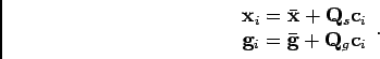
At this stage, each of the images should be aligned to fit a common space. In practice, that space is implicitly defined by the mean shape. Rigid (or Euclidean similarity) transformations, namely translation, scale and rotation, are not always sufficient to warp all images into that common space. Nonetheless, it is crucial that good fitting is obtained before the sampling of grey-level begins. Following these basic transformation which align all images, the displaced control points of each image contain shape-normalised patches. These patches are available for construction of texture vectors and Barycentric arithmetics, which often gets applied to computer graphics and stereo vision, is used to describe the location of all corresponding points. This location is affected by the warps applied to shift a given shape into the space of the mean shape. Triangle meshes are created by stretching lines between neighbouring control points and intensity values are captured one by one (along a chosen grid of points to be samples) and stored in a vector of texture. Each component in such a vector captures the intensity (or colour) of one single pixel as was learned from the examples. Statistical analysis as the one above results in the following formulation for texture:
| (2.2) |
The use of the algorithm above implies that for short vectors and a low number of pixels sampled, noncontinuous appearances will be too easy to spot. In fact, objects will often appear to be nothing more than a collection of polygons that do not quite resemble realistic appearances8. To compensate for this, algorithms from the related field of computer vision can be used, e.g. Phong and Gouraud shading. In practical use, geodesic interpolation is used and the results can be quite astounding considering the low dimensionality of the data.
The models above (2.1, 2.2) are expressed both linearly and compactly - a highly desirable and manageable form. This is due to PCA which reduces the length of the vectors describing shape and texture. Although Eigen-analysis is involved in the process, it is not essential for the understanding of PCA which works as follows.
It is possible to visualise the data as points in a high dimensional
space as was earlier argued. By placing all images in that space,
it is expected that some cloud of points will be present at a specific
somewhat confined region. The breadth of this region or the size of
that cloud will depend on the variation amongst the images (or more
generally data) that is being visualised. PCA obtains the eigenvectors
and eigenvalues of that cloud of points. The highest eigenvalue will
correspond to the most significant eigenvector (see the single-headed
arrow in Figure 3). It indicates the direction that best distinguishes
the image data and is expected to be the longest one too - that is
- the one whose magnitude is the greatest. This is in fact what is
considered to be the principal component which describes that data.
In a recursive manner, at each stage in the process, the principal
component is saved and put aside until only negligible components
are present. The recursion will therefore deal with simpler, more
uniform data as more and more principal components are set aside and
leave a data of lower dimensionality. A smaller number of components
can then be used to express the variation up to a relatively high
level of fidelity. The process is lossy, but so are some other stages
in model construction including the choice of a finite number of landmarks.
That loss is controlled in the sense that one can choose the minimal
amount of variation that must be accounted for9. PCA is used to gain speed while retaining the best descriptors of
variation and difference in shape and intensity. What this all comes
down to is the acquisition of a model that is smaller in size and
is easier to deal with.
The two components
![]() and
and
![]() above need to be
merged to establish a model that accounts for both types of variability
(shape and intensity) and holds within it the correlation between
the two.
above need to be
merged to establish a model that accounts for both types of variability
(shape and intensity) and holds within it the correlation between
the two.
The parameters
![]() and
and
![]() are aggregated
to form a single column vector
are aggregated
to form a single column vector
 |
(2.3) |
It is in some sense a simple concatenation of the two. However, since the values of intensity and shape can be quite different in nature and granularity, some weighing is strongly recommended. If no weighing is applied, then the spread of the points in space is quite undesirable and the components to be identified by PCA are not as beneficial as they would be otherwise. If some values are far greater than others, vicinity takes a turn for the worse and the cloud might be elongated instead of nearly spherical (a 3-D analogy). For rather spherical spreads (or those of almost homogeneous variation), a greater number of large components will be available for selection. Consequently, the variation expressed by a fixed and constant number of principal components will be higher.
A weighing matrix that resolves the problem introduced above is by
convention named
![]() (
(![]() corresponds to shape
as by default this matrix scales the shape parameters only). The form
in which coordinates are stored in
corresponds to shape
as by default this matrix scales the shape parameters only). The form
in which coordinates are stored in
![]() depends on the accuracy
required (e.g. integer and floats), the image size and the number
of dimensions whereas for grey values this form is dependent on the
number of bits used per pixel10. With weighing in place, the aggregation would take a form such as
depends on the accuracy
required (e.g. integer and floats), the image size and the number
of dimensions whereas for grey values this form is dependent on the
number of bits used per pixel10. With weighing in place, the aggregation would take a form such as
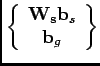 |
(2.4) |
where
![]() is chosen to minimise inconsistencies due
to scale. Lastly, by applying a further PCA to the aggregated data,
the following combined model is obtained:
is chosen to minimise inconsistencies due
to scale. Lastly, by applying a further PCA to the aggregated data,
the following combined model is obtained:
 |
(2.5) |
The appearance is now purely controlled by the parameters
![]() and there is no need to choose values for two families of distinct
parameters as before. This combined model has the benefits of the
dimensionality reduction performed which is based on shape as well
appearance. This means that it now encompasses all the variation learned
and the correlation between these two distinct components. Since PCA
was applied, the number
and there is no need to choose values for two families of distinct
parameters as before. This combined model has the benefits of the
dimensionality reduction performed which is based on shape as well
appearance. This means that it now encompasses all the variation learned
and the correlation between these two distinct components. Since PCA
was applied, the number ![]() of parameters
of parameters
![]() is expected
to be smaller than the number of
is expected
to be smaller than the number of
![]() and
and
![]() put together.
put together.