Method

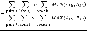
The first of the proposed methods for assessing registration uses a generalisation of Tanimoto's spatial overlap measure [7]. We start with a manual mark-up of each image, providing an anatomical/tissue label for each voxel, and measure the overlap of corresponding labels following registration. We represent each label using a binary image, but after warping and interpolation into a common reference frame, based on the results of NRR, we obtain a set of fuzzy label images. These are used to compute the generalised overlap score [1] as follows:

O $\displaystyle = \frac{ \displaystyle\sum\limits_{\mbox{\small pairs},k}\: \sum\... ...abels},l}\alpha_{l} \sum\limits_{\mbox{\small voxels},i} MAX(A_{kli},B_{kli}) }$

(1)

where

indexes voxels in the registered images,

indexes the label and

indexes image pairs. $A_{kli}$ and $B_{kli}$ represent voxel label values in a pair of registered images and are in the range [0, 1]. The

and

operators are standard results for the intersection and union of a fuzzy set. This generalised overlap measures the consistency with which each set of labels partitions the image volume. The parameter $\alpha_{l}$ affects the relative weighting of different labels. With $\alpha_{l}=1$ , label contributions are implicitly volume weighted with respect to one another. We have also considered the cases where $\alpha_{l}$ weights for the inverse label volume (which makes the relative weighting of different labels equal), where $\alpha_{l}$ weights for the inverse label volume squared (which gives labels of smaller volume higher weighting) and where $\alpha_{l}$ weights for a measure of label complexity (which we define arbitrarily as the mean absolute voxel intensity gradient in the label).

**Figure 1:** The effect of varying the first model parameter of a brain appearance model by $\pm 2.5$ standard deviations.
[scale=0.6]../EPS/brain_0_cps.png

**Figure 2:** Training set and model in hyperspace
[scale=0.25]../EPS/clouds.png

The second method assesses registration in terms of the quality of a generative statistical appearance model, constructed from the registered images. The idea is that a correct registration produces an anatomically meaningful dense correspondence between the set of images, resulting in a better statistical appearance model. We define model quality using two measures - specificity and generalisation [18]. Both are measures of overlap between

Registration is then evaluated through specificity and generalisation ability [18] of the model, or the ability of the model to i) generate realistic examples of the modelled entity and ii) represent well both seen and unseen examples of the modelled class. In practice, these are evaluated by using generative properties of the model to produce a large number of synthetic examples (in this case brain images) that are then compared to real examples in the original set using some pre-defined image distance measure. Minimum distances of synthetic examples to examples in the original set and vice versa, give model specificity and generalisation respectively. Image distance is measured as a mean shuffle distance, or minimum Euclidean distance between a pixel in one image and a corresponding neighbourhood of pixels in the other.

**Figure 3:** The calculation of a shuffle difference image
[scale=0.6]../EPS/shuffle_white_lines.png

**Figure:** Shuffle distance evaluation: **Left:** one image, **Right:** another image, **Centre, from left to right:** images showing contributions to shuffle distance, for $r = 0\:$ (abs. diff.) $,\:1.5,\: 2.1$ & respectively.
[scale=0.22]../EPS/shuffle_dist_example_lighter_shades.png

**Figure 5:** Behaviour of proposed metrics with increasing registration perturbation: a) Generalisation, b) Specificity and c) Tantimoto overlap
[scale=0.5]../EPS/BW_MIAS_overlap_label.png [scale=0.5]../EPS/BW_MIAS_generalisation.png [scale=0.5]../EPS/BW_MIAS_specificity.png

To test the validity of the proposed methods, the brain images were annotated with 6 tissue classes including gray, white matter and CSF that provided the ground truth for image correspondence. Initially, the images were brought into alignment using an NRR algorithm based on the MDL optimisation. A test set of different registrations was then created by applying random perturbations to each image in the registered set using diffeomorphic clamped-plate splines. By choosing a different perturbation seed for each image and gradually increasing the magnitude of the perturbations, a series of image sets of progressively worse spatial correspondence and thus registration quality were obtained. By measuring the quality of the registration at each step, the proposed registration assessment measures can be validated.