PDF version of this document

Results

Model-based algorithms result in appearance models whose determinant is by orders of magnitude lower than that which is measured at the start. The execution time they impose is inferior to MI, much as we expected all along, but is superior to that of MSD.

Since many of the statistics we gathered could indicate that we achieved what we had set our program to do, we intend to apply the same concepts to 2-D and 3-D data in the future. The principles remain unchanged and the only required extension is that of CPS to a higher-dimensional space - something we have developed already. The only foreseeable hindrances will then be the speed of execution and the diligent selection of knot-points for transformation.

Fig. 2. Overlaid plots showing the quality of the appearance model resulting from each objective function.

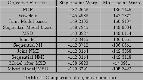
For the results in Figure 3, the number of iterations was set to 50. For single-point transformations, the placement of the control point was random (both in location and magnitude) and for multi-point transformations the positioning of points was made random to abstain from data-bias or advantageous a-priori knowledge. The number of data instances was kept high at 20 in order to allow a substantial group-wise optimisation to be investigated. Objective functions based on mutual information remain flat simply due to the continuity of the data and the fact that it is one-dimensional. The table below shows the different values of ${\displaystyle log\prod}\lambda$. $\lambda$ are the eigenvalues derived from the covariance matrix of the appearance model which was constructed from all 20 data instances. For completeness, differentiation is provided for optimisations which reparameterise over all dimensions at once (joint) or do so separately (sequential).