Progress Report

December 20^th, 2005

Work Agreed Upon

• Liwei et al. - learn more about IMED
• Closest intensity match and distance of exact pixel match
• Entropy-based overlap estimation:
  • Mind subsets, avoid 1000x1000 comparisons
  • See papers for equations (Alpha-Jensen dissimilarity in particular)
  • Possibly slice sets to handle 37x37 images apart
  • Understand the relations to what we do already
• kNN approach (including sum/mean of all image distances)

Work Agreed Upon - Ctd.

• Eye on 3-D, efficiency
• Ponder use of data overlap to extend the training set (skepticism looms over)
• Journal paper draft needs further progress
• Steve Williams - set day for presentation; consider Monday meetings

Paper Draft: Text and Graphics

• Slight changes and addition of figures to TMI draft
• Contacted Bill about our journal submission
  • He intends to submit a paper purely on the overlap measures applied to a segmentation problem and containing a little more theory than was at MICCAI
  • Hoping the two together will make a nice pair of papers for the special edition

Paper Draft - Ctd.

• More work on the document to be done over Christmas
• Ought to expand the explanations, make them clearer, make the flow of arguments better, improve or replace figures (perhaps re-running experiments) and make many other changes
• The document is nowhere near "ready" or in a self-contained state
• Steve Williams: A Monday talk might be used as replacement for the student presentations session - similar content to MIAS-IRC/ISBI

Break-down of Evaluation (Assessment) Approaches

• Image distance:
  • Exact match distance/IMED - Standardising transform - effect is similar to that of smoothing
  • Euclidean, shuffle distance - mind the problem of that notorious initial 'dip'
• Clouds overlap:
  • Minimum distance
  • kNN (k as high as desired, e.g. all graph nodes)
  • Entropy in graphs

Data Annotation and MIAS-Grid

Notes below are somewhat of an utter dross.

These have been added nonetheless to encourage a discussion.

There is an annotation associated with brain images. Point files: stored in a format which is not overly complex. It is built for easy parsing by the corresponding C/C++ code. Example is in the next slide.

Data Annotation and MIAS-Grid

version: 1
n_points: 163
{
118.833 102.5
117.492 100.992
116.333 98.977

[omitted]

104.363 29.637
116.742 26.258
}

Data Annotation and MIAS-Grid - Ctd.

'Version' is there just in case the format gets extended. The number of point is the number of 2-D points contained within the file. You then have pairs of numbers (in this case 163 of them) , which are pixel positions (X,Y) in the corresponding brain images. For each brain, there is one points file. The order of the numbers matters. It defines the correspondence. For example, the 10th point in one file corresponds to the 10th point in another. There can be hundreds of such files, which should typically go under a filename with the extension .pts

Data Annotation and MIAS-Grid - Ctd.

What determines the number of points in the files is a statement in line 2 of each file, e.g.: n_points: 163.

This number indicates exactly how many points are listed inside the subsequent brackets.

Points in the file often correspond to/are embedded in sharp edges and corners, e.g. points around the skull.

A registration algorithm is intended to give an annotation file that is 'correct'. Different registration algorithm could, in some sense, produce different annotation files.

Data Annotation and MIAS-Grid - Ctd.

Whether the point list an orderless list is an interesting question. In practice, the order matters. The points are numbered in such a way so that they can be connected without intersecting one another. There is also the triangulation to take account of. If one thinks of the skull, as an observer move from point 1 to 2, t 3 and so forth, the observer is probably just 'travelling' around the exterior of the head.

Data Annotation and MIAS-Grid - Ctd.

Misunderstanding related to the interpretation of the term "annotation".

Alan needed the label images.

The corresponding control points are indeed another kind of annotation.

One needs the topology of the triangulation to interpret point files in the same manner.

Data Annotation and MIAS-Grid - Ctd.

There is also another obvious issue: both types of annotation are special cases of a generic class. Different representations of the same thing are possible.

The annotations are binary images which represent the existence or inexistence of an anatomical structure, namely left/right ventricle, white matter, grey matter, and the caudate nucleus.

We have 37 such images.

Data Annotation and MIAS-Grid - Ctd.

The numbers in directory names are arbitrary and they simply stand for something that people at MGH used as ID's. There is no notion of control points. Each image in the directory /caudate_right, for example, shows the right caudate nucleus in white. Black color in the image is anything that is not the right caudate nucleus.

In the binary images you can see somewhat of a contour of the label. Think of such anatomical label as if it is represented by just the 'line' which surrounds it. The line, in turn can be sampled using a set of points. That is what the points are. They are usually a description of a label boundary.

Data Annotation and MIAS-Grid - Ctd.

In our case, we always deal with these anatomical structures.

In our experiments, the list which includes 8 structures is the full one.

There is only one point list; each corresponds to an original brain image.

Annotation can come in one of two forms: label images or a point list. Point lists can be ignored altogether.

Data Annotation and MIAS-Grid - Ctd.

The points represent locations in the image which are meaningful and distinguishable.

One can think of them as a poorer method of annotating images.

Labels are much more effective, but are more difficult to obtain.

Unrelated note: all VXL code was resent to Katy for re-compilation

kNN in Calculation of Model Indices

• There appear to be merits to exploring kNN a bit further (see image in subsequent slide for evidence)
• The standard deviation will be smaller
• Hence the error should be smaller too, which gives better sensitivity
• It's the effect on the errors and thus on the sensitivity that was always going to be the only possible interest

kNN in Model Evaluation

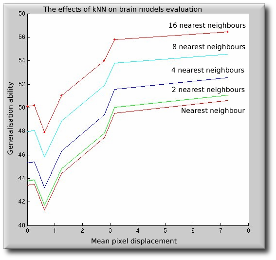
kNN-based Generalisation ability of degrading registration

Image Distances: A Greedy Approach

• We would like to see the entropic measure and possibly replace Euclidean/shuffle by the approach of Liwei et al.

I was following the general approach that was named IMage Euclidean Distance (IMED). I relied on a gross implementation though. It took into account angles and locations of pixels to infer image distances. Instead of assuming a hyperspace with orthogonal axes, where each axis corresponds to one image position (x,y), we took into consideration their spatial relationships. Think of Euclidean distance in the image (between pixels) rather than the space images get embedded in.

Image Distances Greedy Approach - Ctd.

• Shown in the next slides are:
  • Binary(*) images which show, for a given level of grey, positions where that greylevel is believed to lie in. This is based on analysis in the horizontal and vertical axes, as well as the diagonals (8 cases in total, not 4).

(*) not fuzzy at the moment, but in principle, this would be easy to extend.

Image Distances Greedy Approach - Ctd.

• Shown in the next slides are also:
  • Image that shows, for every given pixel, its distance from a given grey level (in this case 20). Efficiency is poor at the moment, so it takes over 15 minutes to generate one such image. We need compute 255x1037 such images, but we haven't got 66,108 hours of computer power to spare (let us not think about 3-D, yet). I'll work on efficiency as we are currently on complexity O(N⁴), just because I wanted to get previews quickly.

It will be very intersting to see how this compares with the shuffle distance. There are some free parameters to tweak, such as how to treat infinite distances. I haven't got around to thinking about it yet.

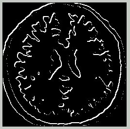
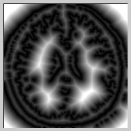
The Nearest Pixel Match Approach

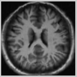
A brain in its original (unwarped) state

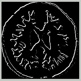
Nearest Pixel Map - 20/255

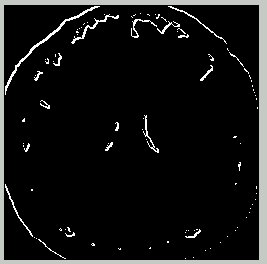
Left: arbitrary brain image; Right: predicted location of intensity with value 20

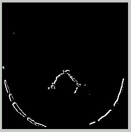
Nearest Pixel Map - 57/255

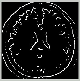
Left: arbitrary brain image; Right: predicted location of intensity with value 57

Nearest Pixel Map - 70/255

Left: arbitrary brain image; Right: predicted location of intensity with value 70

Nearest Pixel Map - 100/255

Left: arbitrary brain image; Right: predicted location of intensity with value 100

Nearest Pixel Map - 150/255

Left: arbitrary brain image; Right: predicted location of intensity with value 150

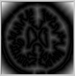
Distance Map to Nearest Intensity Match - 20/255

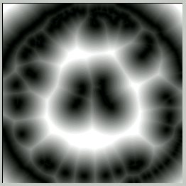
Left: first brain image from the set; Right: distance for each pixel from a pixel of value 20

Distance Map to Nearest Intensity Match - 60/255

Left: first brain image from the set; Right: distance for each pixel from a pixel of value 60

Distance Map to Nearest Intensity Match - 100/255

Left: first brain image from the set; Right: distance for each pixel from a pixel of value 100

The Effects of Dimensionality

(Carole) Could we say anything sensible about the way we would expect our measures to vary with the number of generated examples? This proved to be hard, especially due to the high dimensionality.

Entropic Measures - Discussion

Notes by CJT:

• Estimating entropy from minimal graphs is extremely relevant
• Awareness of it in the context of MI
• Deals more generally with measures of similarity between distributions
• MI is a measure of the (dis)similarity between the jointdistribution and the product of the marginals

Entropic Measures - Discussion - Ctd.

• If we had similarly sized samples of training and synthetic images we could, for example, use the alpha-Jensen Dissimilarity measure directly.
• On the other hand, the path lengths we are currently measuring are clearly sensible estimators of something.
• We need to understand what exactly they are measures of, and whether there are sensible combinations that have more easily interpretable meaning.
• The paper certainly tells us how to normalise things so we are producing normalisable measures of the entropy of something

Entropic Measures - Discussion - Ctd.

The best I can do so far is to point out that under the null hypothesis (the two distributions are the same) what we are measuring (in both the specificity and generalisation cases) is a monotonic function of the entropy of the common distribution.

This might lead us to consider a natural measure such as the difference between the entropy estimated from the A->B nearest neighbour (NN) graph (based on the length we currently compute for specificity), and that measured from the A->A NN graph -- where A is the synthetic set, and B the training set.

Entropic Measures - Discussion - Ctd.

Computed the A->A NN graph overnight. The B->B NN graph takes less than an hour to compute, so can ultimately code up the entropic expression and get the figures. This gives us a measure of overlap that is apparently sensitive. As we need to repeat this several times (e.g. 8), it takes a while to find out if it was all worthwhile.

However, we could just sample from the A->A graph. In practice, the first 18 examples were taken, which is not a wise choice (in retrospect)

Entropic Measures - Discussion - Ctd.

We can increase the sample whenever required or when time permits. It is built in a way which allows it to expand and the measures to becomes more accurate, i.e. depend on a greater proportion of the data in its entirety.

Entropy-based Overlap Estimation

• Got the entropy function in place
• Also computed distances distance all images in the training set
• For the synthetic set, use a subset
• To test the effect of set sizes on the entropy, I have run the following simple test
• In the snippet shown in the next slide:
  • randperm(n): random permutation of the integers from 1 to n
  • entropy: entropy of the row vector

Entropy-based Overlap Estimation - Ctd.

Entropy-based Overlap Estimation - Ctd.

• We certainly have a reason to believe that we must take into account the size of the sets
• The alpha-Jensen dissimilarity measure defines p and q (or Alpha), which we need to set appropriately. It is currently set to 0.5
• Can compare an entropic measure against Generalisation and Specificity.

Progress on Entropic Graphs

• Implemented the alpha-Jensen dissimilarly measure
• Computed the required values for our original IBIM data.
• Facing two issues at the moment
  • Compensation for set size (normalisation). It is hard to judge how effective it is at the moment.
  • The shuffle distance algorithm was not the 'symmetric' type, which is already implemented. It takes twice as long to compute. The symmetric version gives less biased results (distances are not computed in just one direction), yet there are no apparent sensitivity gains.

Progress on Entropic Graphs - Ctd.

We have an entropic method for estimating graph overlap, thus model and registration quality. To get some graphs, we will need to have run large evaluations overnight because of the matrix sizes and the code which is inefficient and interpreted rather than compiled and run.

Entropic Graphs in NRR/Model Assessment

• Early results are available, having processed all the data
• Level of confidence in the algorithm is low
• Generalisation and Specificity included for rough comparison
• Measures appear quite well-correlated

Entropic Graphs in NRR/Model Assessment - Visual

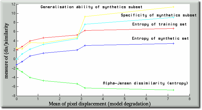
Entropic graph-based evaluation and comparion with other measures and intermediate steps

Next Experiment - Alternative Approach

• Another entopic measure that is in fact simpler
• H(G{A->B])-H(G[A->A]), where G[x->y] is the NN graph of x onto y
• Should be simple to investigate because all the necessary code and data is already in place

Summary and/or Milstones Ahead

• Discussion on point-based annotation and label-based annotation
• Entropy-based method for data cloud overlap
• kNN-based graph analysis
• Journal paper draft
• Extension to 3-D