 PDF version of this entire document
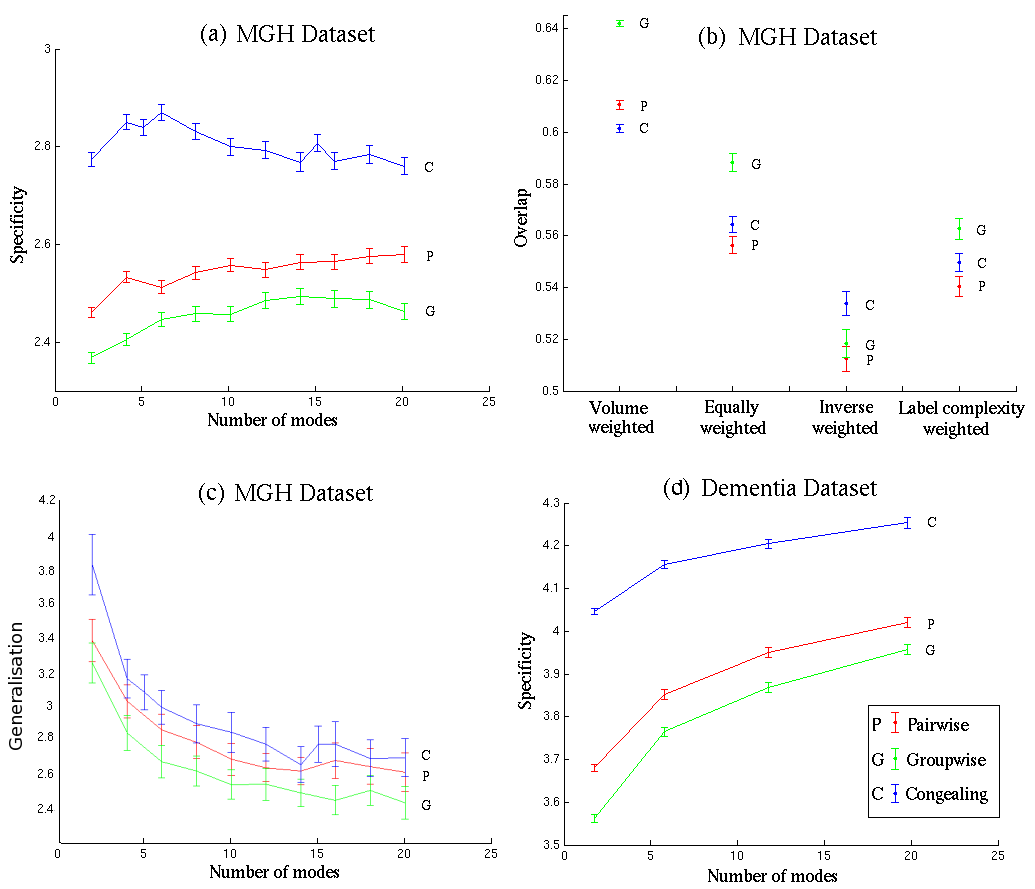
Figure ![[*]](/IMG/latex/crossref.png) compares the performance of the three registration algorithms outlined in Section
compares the performance of the three registration algorithms outlined in Section ![[*]](/IMG/latex/crossref.png) . All the measures tested in the previous section were computed, but results are shown for only the most sensitive model-based method. Figures
. All the measures tested in the previous section were computed, but results are shown for only the most sensitive model-based method. Figures ![[*]](/IMG/latex/crossref.png) (a) and (d) show Specificity calculated using a shuffle radius of 2.1, for different values of
(a) and (d) show Specificity calculated using a shuffle radius of 2.1, for different values of ![]() , the number of modes used to build the generative model. Figure
, the number of modes used to build the generative model. Figure ![[*]](/IMG/latex/crossref.png) (b) shows generalised overlap using different weightings and Figure
(b) shows generalised overlap using different weightings and Figure ![[*]](/IMG/latex/crossref.png) (c) shows Generalisation.
(c) shows Generalisation.
It can be seen that, based on the MGH Dataset, Generalisation as a measure does not provide a separation as useful as that of Specificity. The error bars are larger. This is expected because the size of the training set is small compared to the size of the synthetic set. Nonetheless, both Generalisation and Specificity show a similar behaviour.

|
The response to an increase in the number of modes demonstrates that while it does not significantly affect the merit of the method, relative values may vary. In the case of the MGH Dataset, Specificity goes up as a function of the number of modes, but only for MDL groupwise and pairwise. These two methods seem better suited for the task of brain registration, unlike congealing, which is also suitable for other tasks. The response to change in the number of modes is more pronounced in the case of Generalisation, which unsurprisingly decreases as a function of the number of modes. The curves flatten and reach a plateau at around 14 modes. In order to properly occupy a space with the set of synthetic images, a larger number of modes may therefore be necessary.
The results shown in Figures ![[*]](/IMG/latex/crossref.png) (a) and (c) suggest that the MDL groupwise approach gives the best registration result for the MGH Dataset, followed by Pairwise and Congealing in order of decreasing performance - irrespective of the value of
(a) and (c) suggest that the MDL groupwise approach gives the best registration result for the MGH Dataset, followed by Pairwise and Congealing in order of decreasing performance - irrespective of the value of ![]() . The error bars in the case of Specificity show that the differences are statistically reasonable in the sense that they leave a significant gap between the 3 methods; the same cannot be said about Generalisation where error bars intersect.
. The error bars in the case of Specificity show that the differences are statistically reasonable in the sense that they leave a significant gap between the 3 methods; the same cannot be said about Generalisation where error bars intersect.
The results for Generalised Overlap, shown in Figure ![[*]](/IMG/latex/crossref.png) (b), are more complicated, with the performance of the different NRR algorithms ordered differently for different weightings. Overall, the same general pattern emerges as for Specificity, with the Groupwise method generally best (statistically significantly in two cases), but with no significant difference between Pairwise and Congealing in most cases. The results for inverse volume weighting generally lack significance, but are inconsistent with those obtained using the other weighting schemes. Volume weighting gives the best separation between the different variants, and places the three methods in the same order as Specificity. Overall, this supports the interpretation that Specificity give results that are generally equivalent to those obtained using Generalised Overlap, but with higher sensitivity. Finally, the Specificity results shown in Figure
(b), are more complicated, with the performance of the different NRR algorithms ordered differently for different weightings. Overall, the same general pattern emerges as for Specificity, with the Groupwise method generally best (statistically significantly in two cases), but with no significant difference between Pairwise and Congealing in most cases. The results for inverse volume weighting generally lack significance, but are inconsistent with those obtained using the other weighting schemes. Volume weighting gives the best separation between the different variants, and places the three methods in the same order as Specificity. Overall, this supports the interpretation that Specificity give results that are generally equivalent to those obtained using Generalised Overlap, but with higher sensitivity. Finally, the Specificity results shown in Figure ![[*]](/IMG/latex/crossref.png) (d) for the Dementia Dataset, place the three methods in the same order.
(d) for the Dementia Dataset, place the three methods in the same order.
A single comparison, as presented in this chapter, took a few hours to complete on a modern computer. The experiments reported were performed in 2-D to limit the computational cost of running the large-scale evaluation for a range of parameter values and with repeated measurements. The extension to 3-D is, however, trivial, though the calculation of shuffle distance for 3-D images increases the computational cost significantly. The method in 3-D has been implemented and the time taken to evaluate the registration of 100 190x190x50 images using a shuffle radius of 2.1 and
![]() is around 62.5 hours on a modern PC. The next section looks at preliminary experiments which show the program's operation once I added 3-D support to it.
is around 62.5 hours on a modern PC. The next section looks at preliminary experiments which show the program's operation once I added 3-D support to it.
Roy Schestowitz 2010-04-05