 PDF version of this entire document


Correspondence-by-optimisation requires an objective function that
provides a measure of model quality for a given set of correspondences.
In early work, Kotcheff and Taylor [] proposed the use
of the determinant of the shape covariance matrix (
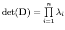 )
as a measure of model quality, arguing that a good correspondence
should result in a model with a small distribution in shape space.
They showed encouraging results but did not provide a sound theoretical
justification for the approach.
)
as a measure of model quality, arguing that a good correspondence
should result in a model with a small distribution in shape space.
They showed encouraging results but did not provide a sound theoretical
justification for the approach.
There are other issues with this approach. When generating something simple like a 2-D distribution of points, it is trivially possible to show what happens if the determinant changes and one simple way to do this is by generating data from a 2-D distribution, then looking at the determinant as noise is added to the point positions. As the distribution changes, the determinant changes too, but a key issue is the need to prevent small modes from almost zeroing the determinant. Later on in this chapter I will discuss a solution to this.
The key deficiency with determinant as a parameter is that it is a bit arbitrary, so Davies et al. [] built on this work, providing the MDL objective function. With MDL, their basic idea was that a good model ought to allow a simple description of the training set - in an information theoretic sense. This MDL objective function estimates the information (in bits) required to encode two parts of the coding scheme, namely the parameters of the model and the training set of shapes encoded using that model. Model parameters are related to the number of model modes (degrees of variation) and the second part scales in proportion to the number of examples in the training set. In cases where the training set is large, that latter component dominates and outweighs the former, in which case the use of model determinant as an approximation can be justified, at least for a multivariate Gaussian [].
For one-dimensional models, the shapes and models were encoded using an expression that considers the family of such distributions and is computed by summing two parts; the description length for encoding value and accuracy of a parameter along with the description length for encoding the value itself using the model. To transmit a one-dimensional model, one needs to calculate, based on Shannon Coding codeword length [], a statistical model with event probabilities. This was done by quantising the centered data set and instead obtaining a set of discrete events. To code the parameters, one must also consider the accuracy in order for a receiver of the message to be able to decrypt it. The total code length was the sum of the lengths of the data describing parameter accuracy and the quantised parameters. It was also necessary to code the data itself. In this case of a model, what remained was an accumulation of the following components:
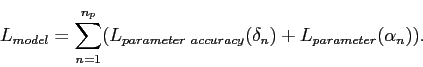
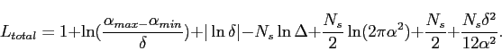
The MDL objective function has been discussed in an abstract form
so far, along with some various steps in its derivation, but to formulate
it symbolically (where ![]() represents description length):
represents description length):
| (4.1) |
Breaking it down further, let us suppose a full description of our model means specifying a set of ![]() parameters
parameters
![]() . To get a finite message length, we obviously can only transmit parameters to some finite number of decimal places (or to some finite accuracy), hence we also have to consider the accuracy of each parameter, call it
. To get a finite message length, we obviously can only transmit parameters to some finite number of decimal places (or to some finite accuracy), hence we also have to consider the accuracy of each parameter, call it ![]() . The description length for the entire model can then be written as:
. The description length for the entire model can then be written as:
 |
(4.2) |
This is the first component among two and the precise derivation will
be shown here for completeness. The parameters in the first component
(![]() ) are derived and coded as follows.
) are derived and coded as follows.
It is possible, without loss of generality, to consider the case of just a single parameter and drop the subscript for clarity. What actually gets transmitted is not the raw parameter value ![]() , but the quantized value
, but the quantized value ![]() , described to an accuracy
, described to an accuracy ![]() , that is:
, that is:
| (4.3) |
| (4.4) |
Since there is no prior knowledge in this case, the distribution of
![]() over this range is assumed to be flat, which gives
the codeword length:
over this range is assumed to be flat, which gives
the codeword length:
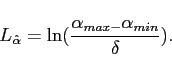 |
(4.5) |
The receiver of this cannot decrypt the value of ![]() without
also knowing the value of the accuracy
without
also knowing the value of the accuracy ![]() , so the quantisation
parameter
, so the quantisation
parameter ![]() may take the following form:
may take the following form:
| (4.6) |
| (4.7) |
![]() is just the length of the integer
is just the length of the integer ![]() , whereas the additional bit is for encoding the sign of
, whereas the additional bit is for encoding the sign of ![]() .
The total length for transmitting the parameters is then the sum of
.
The total length for transmitting the parameters is then the sum of
![]() and
and ![]() .
.
There is also the sum over description lengths of training examples
(the second component of the coding formulation). Although this does
not give something which is the absolute minimum length, it takes
a form which is suitable for optimisation. The total description length,
![]() , is the sum of the two parts where for
, is the sum of the two parts where for ![]() shapes
that I arbitrarily call
shapes
that I arbitrarily call ![]() , the second term is:
, the second term is:
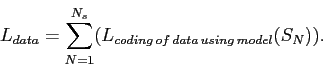 |
(4.8) |
The training examples are encoded as follows. We will consider the case of 1-D centered and quantised data (with quantisation parameter ![]() ),
),
![]() , which is encoded using a 1-D Gaussian
, which is encoded using a 1-D Gaussian
![]() For a bin centered at
For a bin centered at ![]() , the associated probability is:
, the associated probability is:
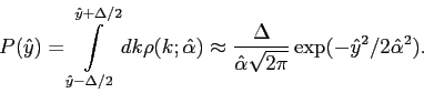 |
(4.9) |
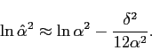
Numerically, it can be shown to be a decent approximation for all
values
![]() , so
, so ![]() is now
just assumed equal to
is now
just assumed equal to ![]() and the code length of the data is
and the code length of the data is
 |
(4.10) |
Then, it is possible to obtain the variance of the quantised data:
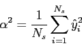 |
(4.11) |
and additionally,
![]()
![]() is still different
from the nearest quantised value
is still different
from the nearest quantised value ![]() so
so
![]() .
.
By averaging over an ensemble of different sets and assuming the distribution
for ![]() is flat over this range, it is found that:
is flat over this range, it is found that:
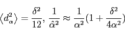 |
(4.12) |
and
 |
(4.13) |
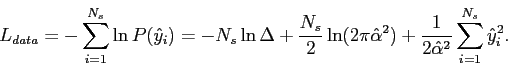
Finally, by combining these expressions, it turns out that description length of the data is
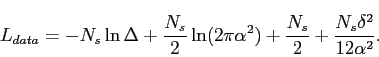 |
(4.14) |
and so
 |
(4.15) |
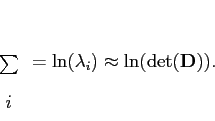
It is worth noting that the MDL objective function includes the term
![]() (the variance), which is closely related to Kotcheff
and Taylor's [] determinant of the model covariance
matrix (product of eigenvalues, or
).
The latter often dominates and is a lot cheaper to compute. In essence,
(the variance), which is closely related to Kotcheff
and Taylor's [] determinant of the model covariance
matrix (product of eigenvalues, or
).
The latter often dominates and is a lot cheaper to compute. In essence,
![]() and as
and as
![]() , for more directions (a multivariate
rather than a 1-D Gaussian) the term would be
, for more directions (a multivariate
rather than a 1-D Gaussian) the term would be
 |
(4.16) |
There are more details about this relationship in []. Since the determinant roughly measures the volume which the training set occupies in space, this favours compact models. The description length of this determinant is
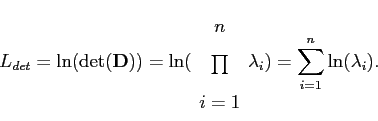 |
(4.17) |
The definition of the covariance matrix itself was given in Chapter
3 in the context of PCA. In Chapter 3, ![]() was also defined to be
the number of modes and
was also defined to be
the number of modes and ![]() here is the number of modes fitting the
expression. This MDL objective function can be conveniently approximated
by the determinant-based objective function, so my methods will be
inspired by it. One of the deficiencies, as Chapter 5 will explain,
is that the determinant - being a product - can be negatively affected
by tiny eigenvalues.
here is the number of modes fitting the
expression. This MDL objective function can be conveniently approximated
by the determinant-based objective function, so my methods will be
inspired by it. One of the deficiencies, as Chapter 5 will explain,
is that the determinant - being a product - can be negatively affected
by tiny eigenvalues.