PDF version of this entire document
Model construction with the aid of PCA is far from new and it is inspired
by other strands of work [17]. In prior work which delved
into face modeling Cootes et al. found the mean shape and restricted
set of PCA axes that provide a concise description of the training
set of shapes. This was used to build a 2-D model of shape and this
model could also be used to generate new shapes. Let such a new shape
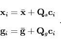
be x, generated from a set of shape parameters
![]() :
:
The matrix
![]() contains the eigenvectors of the covariance
matrix of the training data.
contains the eigenvectors of the covariance
matrix of the training data.
The generated shapes can be constrained to be similar to those seen
in the training set by constraining the allowed shape parameters,
![]() , to be similar to those extracted or learned from
the training shapes. Typically, the distribution of training set shape
parameters is modelled by a multivariate Gaussian pdf, and new shapes
are generated by sampling from this pdf. To further enhance this type
of models, appearance models were later developed. The appearance
models encapsulate textural information about the variation across
this set of shapes. It is possible to extend the former method and
construct models that encapsulates not just the variation of the shape
of objects in images, but also the variation in the appearance of
the object itself. Appearance models were developed by Edwards et
al. []. Their greatest contribution, advantage,
and essence lie within the fact that they incorporate textural information
rather than shape alone. Texture is a made out of grey-level pixel
intensities. Incorporation of full colour is possible as well [].
Colour can be simply thought of as an extension of the single grey-scale
band. It can be divided into bands using the most common separability:
red, green, and blue components6.
, to be similar to those extracted or learned from
the training shapes. Typically, the distribution of training set shape
parameters is modelled by a multivariate Gaussian pdf, and new shapes
are generated by sampling from this pdf. To further enhance this type
of models, appearance models were later developed. The appearance
models encapsulate textural information about the variation across
this set of shapes. It is possible to extend the former method and
construct models that encapsulates not just the variation of the shape
of objects in images, but also the variation in the appearance of
the object itself. Appearance models were developed by Edwards et
al. []. Their greatest contribution, advantage,
and essence lie within the fact that they incorporate textural information
rather than shape alone. Texture is a made out of grey-level pixel
intensities. Incorporation of full colour is possible as well [].
Colour can be simply thought of as an extension of the single grey-scale
band. It can be divided into bands using the most common separability:
red, green, and blue components6.
A shape model can be thought of as providing very limited information about the appearance of an object within an image, in that it describes the shape of an object, where it is implicitly understood that the shape of an object corresponds to strong edges in an image.
Appearance models describe not only the shape of an object, but the image intensities within the outline of the object as well. In the following subsections, three steps are discussed in turn: modelling shape, modelling intensity, and combined models.
The first step is building of shape models, which use a finite number
of modes for representation. Shape models that are built from the
outlines of objects in images enable those images to be brought into
a state of alignment. We can warp the shapes within an image to match
the mean shape. By interpolation, we can extend this warp to the entire
interior of the object. This means that corresponding parts of shapes
in those images will be easy to identify and then use, e.g. in order
to sample intensities. To model texture, differences in shapes are
removed by morphing each training image to the mean shape7. A shape-free texture patch can then be estimated from the image
by sampling on a regular grid and forming a vector ![]() .
Statistical analysis proceeds as for shapes and it results in the
following linear expression for texture
.
Statistical analysis proceeds as for shapes and it results in the
following linear expression for texture
![]() is the intensity vector.
is the intensity vector.
![]() contains the eigenvectors of the covariance matrix of the training
data and
contains the eigenvectors of the covariance matrix of the training
data and
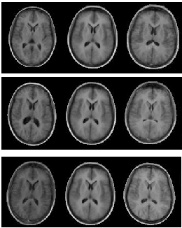
![]() controls the intensity. An example appearance
model is shown in Figure
controls the intensity. An example appearance
model is shown in Figure ![[*]](/IMG/latex/crossref.png) . The process is hardly different
from dimensionality reduction in the case of shape. The models in
Equation and Equation
have a linear form, so they are quite compact. This is a highly desirable
property which makes the models flexible and manageable.
. The process is hardly different
from dimensionality reduction in the case of shape. The models in
Equation and Equation
have a linear form, so they are quite compact. This is a highly desirable
property which makes the models flexible and manageable.
However, at the moment, the two components of the model, namely the
shape ![]() and the shape-free texture
and the shape-free texture ![]() , are
independent. In real images, shape and texture are not necessarily
independent. One simple example to think of is an image of an individual's
face. When the person changes expression, the shape of the face changes.
But the texture (i.e. positions of highlights and shadows) obviously
changes too, in a way that is correlated with the shape change. Hence
it is desirable to merge the shape and texture models, so as to obtain
a new model that is aware of both types of variation. This combined
model can then also incorporate any correlations between shape and
texture.
, are
independent. In real images, shape and texture are not necessarily
independent. One simple example to think of is an image of an individual's
face. When the person changes expression, the shape of the face changes.
But the texture (i.e. positions of highlights and shadows) obviously
changes too, in a way that is correlated with the shape change. Hence
it is desirable to merge the shape and texture models, so as to obtain
a new model that is aware of both types of variation. This combined
model can then also incorporate any correlations between shape and
texture.
The parameters
![]() and
and
![]() are aggregated
to form a single column vector
are aggregated
to form a single column vector
The new vector is a simple concatenation of the two. However, since
the values of intensity and shape can be very different in magnitude,
weighting is needed. Such weighting brings equilibrium, under which
both shape and intensity maintain a sufficiently-noticeable effect
and impact on the model they jointly build. A weighing matrix resolves
the problem introduced here and it is, by convention, named
![]() 8. With weighing in place, aggregation takes the form
8. With weighing in place, aggregation takes the form
where
![]() is set to minimise inconsistencies due to
scale. By applying another PCA step to the aggregated data, the following
combined model is obtained
is set to minimise inconsistencies due to
scale. By applying another PCA step to the aggregated data, the following
combined model is obtained
The appearance (shape and texture) is now purely controlled by the
new set of parameters, ![]() . There is no need to choose values
for two `families' of distinct parameters. This combined model reaps
the benefits of the dimensionality reduction performed, which is based
on shape as well appearance. This means that this new model encompasses
all the variation learned and the correlation between these two distinct
components. Since PCA was applied, the number
. There is no need to choose values
for two `families' of distinct parameters. This combined model reaps
the benefits of the dimensionality reduction performed, which is based
on shape as well appearance. This means that this new model encompasses
all the variation learned and the correlation between these two distinct
components. Since PCA was applied, the number ![]() of parameters
of parameters
![]() is expected to be smaller than the number of parameters in
is expected to be smaller than the number of parameters in
![]() and
and
![]() put together.
put together.
|
The work we shall deal with will not require texture or even a complex
model such as the above. Prior work, however, necessitates understanding
of possible future extensions.
Roy Schestowitz 2012-01-08