Implementation

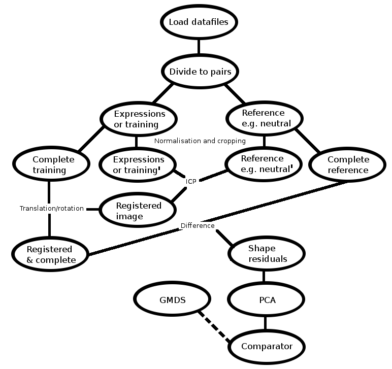
P reparatory stages, such as pre-processing of images, can be done separately from the main experiments as these stages do not change once the algorithm is deemed acceptable. However, the body of the work too can be made more modular and thus explained by its modules or its layers of operation. Taking stock of what we have and organising it visually gives us an overview image, as in Figure $[*]$ . It hopefully helps keep track of the said process, implemented mostly in according with the IJCV reference description.

**Figure:** Program steps broken down into an overview-type flowchart

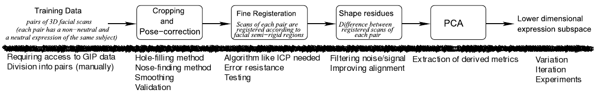
The work on code can be sub-divided into different stages which can also be treated separately in order to make the experimentation pipeline more manageable. We shall classify the stages as follows: preprocessing, modelling, validation, and benchmarks. The key part is about PCA [], which MATLAB implements with http://www.mathworks.com/help/toolbox/stats/princomp.htmlprincomp; it is essential for constructing statistical models, via decomposition of face characteristics as derived automatically from the dataset.

**Figure:** Areplotted block diagram of the components in the IJCV paper (top) and our proposed extension/modifications (bottom), and the already-implemented procedures

Shown in Figure $[*]$ is an annotated version of the original figure from the paper. The overview is simplistic in the interests of abstraction and elegance. For instance, methods of hole removal are described only as local statistics. This leaves room for multiple competing implementations with different results depending on ad hoc refinement (ours was about 3,000 lines of code at the start of April).

The functionality is two-fold; one major part is modeling and the latter, which shares many pertinent components, does the matching. The program first takes as input the training set from which to build a model to be used as a similarity measure (done by Schestowitz et al. for NRR [,,]), which is an overkill that assumes infinite resources like time and RAM. The latter part, which can be scripted to run standardised benchmarks, takes as input a probe and gallery which is assumed to contain just one instance of the same person as in the probe. Initially, two similarity measures are taken. One is residual mean and the other is distance from the N utmost principal axes of the EDM.

For experiments, a control file loops around the algorithm with different datasets and parameters as input. It is worth repeating that the quality of results will largely depend on one's ability to clean up the data - removing the wheat from the chaff (spikes, noise, irrelevant parts of faces) - as that very much determines what an expression is modeled as.

This portion of the document explains to a limited degree the computational methods and puts a lot more emphasis on the software tools.