PDF version of this entire document

New Similarity Measure

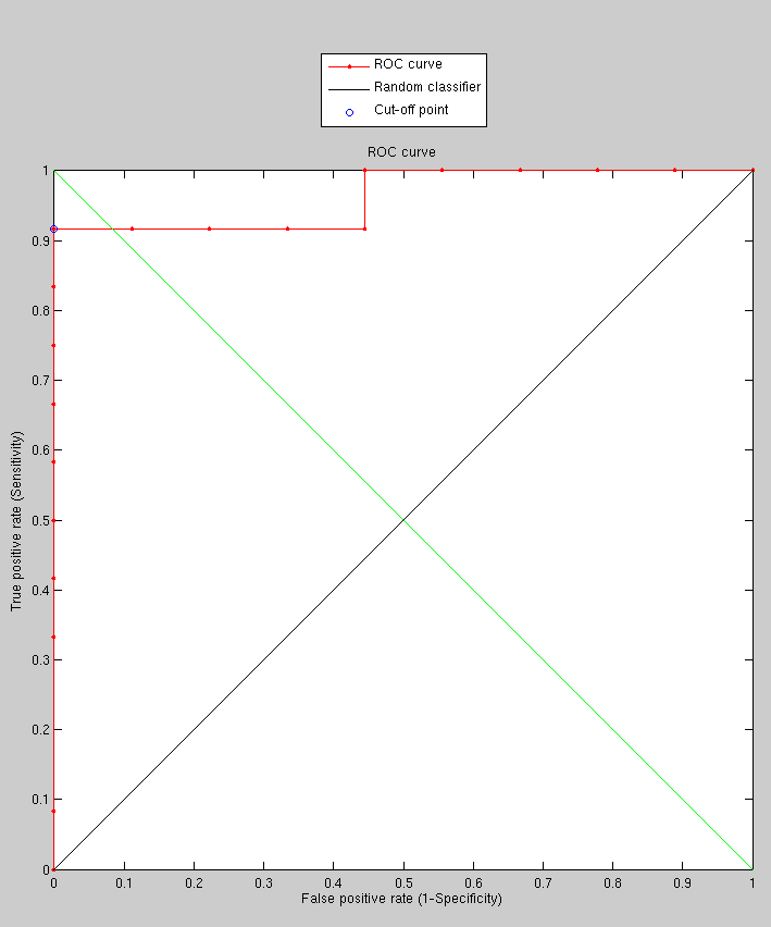
In order to stride forward, another improvement is being explored. Currently, results where similarity is derived from the determinant of the eigenvalues of the covariance matrix seem promising (Figure ). But the experiment was probably too small. It shows training on 170 images with just 22 images being targets. As before, the sets are generally hard and they are picked with expression variation.

Figure: The results of measuring the similarity by determinant of the eigenvalues of the covariance matrix and engaging in a recognition task

Having spent many hours exploring other objective functions (or similarity measures with rigid transformation), the one which tended to work better was applied to a somewhat larger set and with the exception of few images that need to be looked at carefully, recognition in hard cases is basically improved, even with a coarse model. This one experiment samples 8 points apart and uses no smoothing. The next logical step would be to look at the cause for incorrect matching and also test to see the effect of rotation, translation, smoothing, etc. Literature on the subject also suggests how Lambda might be tweaked to account differently for eigenvalues. Results from the experiment are shown in Figure .

Figure: Results of an experiment where the determinant is again being explored, this time with a larger set

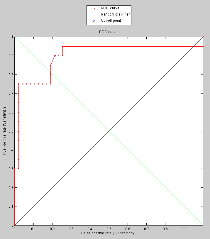
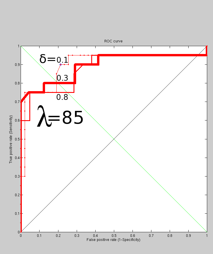
Putting the simple experiment in perspective, Figure shows what happens when $\delta$ is varied in the sense that it is increased. As expected, this weakens the measure because it reduces the impact of zeroes but also weakens the signal. To succinctly explains the point of this measure, it is inspired by Kotcheff's work in the late nineties. It is quite simple to implement and it relies on an implicit similarity measure, which is an approximation of the quality of a model. This model is an aggregate model of known face residuals and a newly-introduced one (the probe). A correct match is one that results in high similarity -and builds a good model, characterised by concision. This observation was exploited to create a similarity measure that is data-agnostic and generalisable.

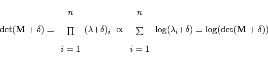
Similarity is computed indirectly in this case. The algorithm does so by calculating the model, namely by looking at the covariance matrix of that model. To efficiently evaluate model complexity, $\sum\limits_{i=1}^{n} \log(\lambda_{i}+\delta)$ is obtained where $\lambda_{1<i<n}$ are the $n$ eigenvalues of the covariance matrix whose magnitudes are the greatest and $\delta$ is a small constant (around 0.1) which adds weight to each eigenvalue. 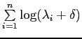This approximates

$$\det(\mathbf{M+\delta)}\equiv\begin{array}{c} n\\ \prod\\ ... ...y}\log}(\lambda_{i}+\delta)\equiv\log(\det(\mathbf{M+\delta}))$$ (6)

where $\mathbf{M}$ is the model's covariance matrix under consideration and $\delta$ is a constant which would quite importantly ensure nothing gets multiplied by 0 or a summation stuck too close to 0. This whole term is an approximation of similarly between images.

In order to test performance for much smaller values of $\delta$ there is a need to limit how many of $\lambda_{1<i<n}$ to remove (those of least magnitude). This will be the next step. Later on, large sets can build better model with data which is easier to deal with and yields better results.

Figure: Results of an experiment where the determinant is again being explored with a comparison of the curves for 3 values of $\delta$