PDF version of this document


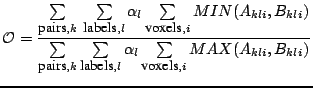
The first of the proposed methods for assessing registration quality uses a generalisation of Tanimoto's spatial overlap measure [1]. We start with a manual mark-up of each image, providing an anatomical/tissue label for each voxel, and measure the overlap of corresponding labels following registration. Each label is represented using a binary image, but after warping and interpolation into a common reference frame, based on the results of NRR, we obtain a set of fuzzy label images. These are combined in a generalised overlap score [5]:
The second method assesses registration in terms of the
quality of a generative statistical appearance model, constructed
from the registered images - for all the experiments reported
here, this was an active appearance model
(AAM) [3]. The idea is that a correct
registration produces an anatomically meaningful dense
correspondence between the images, resulting in a better
appearance model of the anatomy. We define model quality using
two measures - generalisation and specificity. Both
are measures of overlap between the distribution of original
images and a distribution of images sampled from the model, as
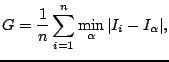
illustrated in Figure 1. If we use the generative
property of the model to synthesise a large set of images,
![]() , we can define
Generalisation
, we can define
Generalisation ![]() as:
as:
 |
(2) |
where ![]() is a measure of distance between
images,
is a measure of distance between
images, ![]() is the
is the ![]() training image, and
training image, and
![]() is the minimum over
is the minimum over ![]() (the set of synthetic images). That is, Generalisation is the average
distance from each training image to its nearest neighbour in the
synthetic image set. A good model exhibits a low value of
(the set of synthetic images). That is, Generalisation is the average
distance from each training image to its nearest neighbour in the
synthetic image set. A good model exhibits a low value of ![]() ,
indicating that the model can generate images that cover the full
range of appearances present in the original image set. Similarly,
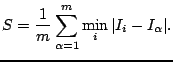
we can define Specificity
,
indicating that the model can generate images that cover the full
range of appearances present in the original image set. Similarly,
we can define Specificity ![]() as:
as:
 |
(3) |
That is, Specificity is the average distance of each
synthetic image from its nearest neighbour in the original image
set. A good model exhibits a low value of ![]() , indicating that the
model only generates synthetic images that are similar to those in
the original image set. The uncertainty in estimating
, indicating that the
model only generates synthetic images that are similar to those in
the original image set. The uncertainty in estimating ![]() and
and ![]() can also be computed.
can also be computed.
In our experiments we have defined ![]() as the shuffle
distance between two images, as illustrated in
Figure 2. Shuffle distance is the mean of the
minimum absolute difference between each pixel/voxel in one image,
and the pixels/voxels in a shuffle neighbourhood of radius
as the shuffle
distance between two images, as illustrated in
Figure 2. Shuffle distance is the mean of the
minimum absolute difference between each pixel/voxel in one image,
and the pixels/voxels in a shuffle neighbourhood of radius ![]() around the corresponding pixel/voxel in a second image. When
around the corresponding pixel/voxel in a second image. When ![]() , this is equivalent to the mean absolute difference
between corresponding pixels/voxels, but for larger values of
, this is equivalent to the mean absolute difference
between corresponding pixels/voxels, but for larger values of ![]() the distance increases more smoothly as the misalignment of
structures in the two images increases. The effect on the
pixel-by-pixel contribution to shuffle distance as
the distance increases more smoothly as the misalignment of
structures in the two images increases. The effect on the
pixel-by-pixel contribution to shuffle distance as ![]() is
increased is illustrated in Figure 3.
is
increased is illustrated in Figure 3.
|
[width=0.9]../EPS/Final/shuffle-example-from-presentation.png
|
|
[width=0.98]../EPS/Carole/shuffle_dist_example_lighter_shades.png
|
|
[width=0.89
]../EPS/Carole/Allthree.png
|