PDF version of this entire document
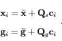
The models in Equation ![[*]](/IMG/latex/crossref.png) and Equation
have a linear form, so they are quite compact. This is a highly desirable
property which makes the models flexible and manageable.
and Equation
have a linear form, so they are quite compact. This is a highly desirable
property which makes the models flexible and manageable.
However, at the moment, the two components of the model, namely the
shape ![]() and the shape-free texture
and the shape-free texture ![]() , are
independent. In real images, shape and texture are not necessarily
independent. One simple example to think of is an image of an individual's
face. When the person changes expression, the shape of the face changes.
But the texture (i.e. positions of highlights and shadows) obviously
changes too, in a way that is correlated with the shape change. Hence
it is desirable to merge the shape and texture models, so as to obtain
a new model that is aware of both types of variation. This combined
model can then also incorporate any correlations between shape and
texture.
, are
independent. In real images, shape and texture are not necessarily
independent. One simple example to think of is an image of an individual's
face. When the person changes expression, the shape of the face changes.
But the texture (i.e. positions of highlights and shadows) obviously
changes too, in a way that is correlated with the shape change. Hence
it is desirable to merge the shape and texture models, so as to obtain
a new model that is aware of both types of variation. This combined
model can then also incorporate any correlations between shape and
texture.
The parameters
![]() and
and
![]() are aggregated
to form a single column vector
are aggregated
to form a single column vector
The new vector is a simple concatenation of the two. However, since
the values of intensity and shape can be very different in magnitude,
weighting is needed. Such weighting brings equilibrium, under which
both shape and intensity maintain a sufficiently-noticeable effect
and impact on the model they jointly build. A weighing matrix resolves
the problem introduced here and it is, by convention, named
![]() 3.4. With weighing in place, aggregation takes the form
3.4. With weighing in place, aggregation takes the form
where
![]() is set to minimise inconsistencies due to
scale. By applying another PCA step to the aggregated data, the following
combined model is obtained
is set to minimise inconsistencies due to
scale. By applying another PCA step to the aggregated data, the following
combined model is obtained
The appearance (shape and texture) is now purely controlled by the
new set of parameters, ![]() . There is no need to choose values
for two `families' of distinct parameters. This combined model reaps
the benefits of the dimensionality reduction performed, which is based
on shape as well appearance. This means that this new model encompasses
all the variation learned and the correlation between these two distinct
components. Since PCA was applied, the number
. There is no need to choose values
for two `families' of distinct parameters. This combined model reaps
the benefits of the dimensionality reduction performed, which is based
on shape as well appearance. This means that this new model encompasses
all the variation learned and the correlation between these two distinct
components. Since PCA was applied, the number ![]() of parameters
of parameters
![]() is expected to be smaller than the number of parameters in
is expected to be smaller than the number of parameters in
![]() and
and
![]() put together.
put together.
|
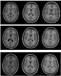
The effect of varying different elements of a combined model ![]() for a model built from a set of 2-D MR brain images is shown in Figure . The number of modes (columns) in
for a model built from a set of 2-D MR brain images is shown in Figure . The number of modes (columns) in
![]() and
and
![]() is one less than the number of images. In practice, it is often possible to approximate images pretty well, using fewer modes
is one less than the number of images. In practice, it is often possible to approximate images pretty well, using fewer modes ![]() .
.
Roy Schestowitz 2010-04-05