Manipulating the Correspondence

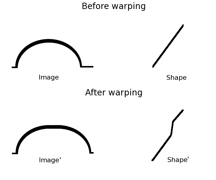
Shape drives the NRR in the sense that manipulating the shape component and then resampling the images makes NRR possible. Each image is sampled at a fixed number of points and shape determines the position of the points that are sampled.

The basic idea is demonstrated in Figure $[*]$ . For a straight diagonal shape curve, each point on the bump is mapped to an identical position after warping because any point along the $\mathbf{x}$ axis in the shape curve coincides with the same value on the $\mathbf{y}$ axis. If the shape curve is altered through warping, then points on the bump are remapped accordingly, based on the new shape curve. In order to build combined models, both components must be taken into account so that variation of shape will be restricted too.

**Figure:** A bump image as shown on the left before warping (top) and after warping (bottom), where the corresponding shape curve on the right hand side is changed so as to help assimilate one bump to another (seen at the bottom left, where reparameterisation based on the shape curve helped widen the bump)

In order to show how 1-D images get registered, it is useful to provide different ways of visualising the data. The videos in the enclosed CD-ROM contain illustrations that are dynamic (time sequences) where warps are repeatedly applied, leading to change over time.

Dealing with several such bumps^5.1 in turn, one can visualise them as shown in Figure $[*]$ and Figure $[*]$ , where bumps are laid side by side. Many of the auxiliary videos depict a 1-D registration using this representation of the data. Figure $[*]$ has these images displayed as surfaces. Since the goal is to align such images, such side-by-side presentation proves helpful.

**Figure:** Bumps being registered. The registration process is visualised by an image composed of data vectors (laid horizontally alongside one another). The columns are 1-D vectors to be interpreted as grey-scale pixels.
$\includegraphics[scale=0.7]{Graphics/image_vectors}$

**Figure:** A larger example of the pixel representation for 1-D bump data.
$\includegraphics[scale=0.6]{Graphics/pixels}$

**Figure:** Original image set depicted in 3-D. A set of size 5 is shown before applying any warps which are intended to align this data.
$\includegraphics[scale=0.3]{Graphics/test_on_target_7-4}$

An original, unwarped image is a function $f(\mathbf{x})$ , where $f(\mathbf{x})$ is sampled at a set of equally-spaced points (which are the pixel set, $\mathbf{x}$ ).

Suppose there is a warp $\phi(x)$ which collapses the unit interval [0,1] onto itself, with no folds or tears. To transform images in this way, it seems reasonable to employ clamped-plate splines because they address such requirements given specific boundaries^5.2. The clamped-plate splines prevent any of the regions in an image from being torn or folded, hence they preserve the existence and integrity of all image regions^5.3.

When the image is warped using biharmonic clamped-plate splines, the set of previously equally-sampled pixel positions will move to new positions $\phi(x)$ and carry their image value with them. Two cases, namely single-point and multi-point warps, were both considered, where in the latter case composition is used to obtain more flexible deformations.

Although the property of height was not intended to be ignored during registration (it is the maximum intensity, which cannot be discarded), it was expected that it would remain unchanged. This is due to the nature of CPS-based warps being used. They are perfectly diffeomorphic^5.4[] provided that their constraints are obeyed. The warps are manipulated by altering the direction and magnitude of a single central knotpoint, or multiple knotpoints. Both cases were considered here and the warps were applied to localised parts of the line, not the entire line.

In the experiments described later, the bumps were all symmetric in the sense that the curves were the same left and right of the centre of the bump. The height,

, took a single value value from a fixed range set {hi, low} where

and

. The data was therefore far simpler than 1-D data which is not constrained in any way. The height of the bump and the position at which the bump grows tall jointly defined the appearance that bump, so two real numbers (a tuple) at the minimum sufficed for the reconstruction of each bump.