PDF version of this entire document
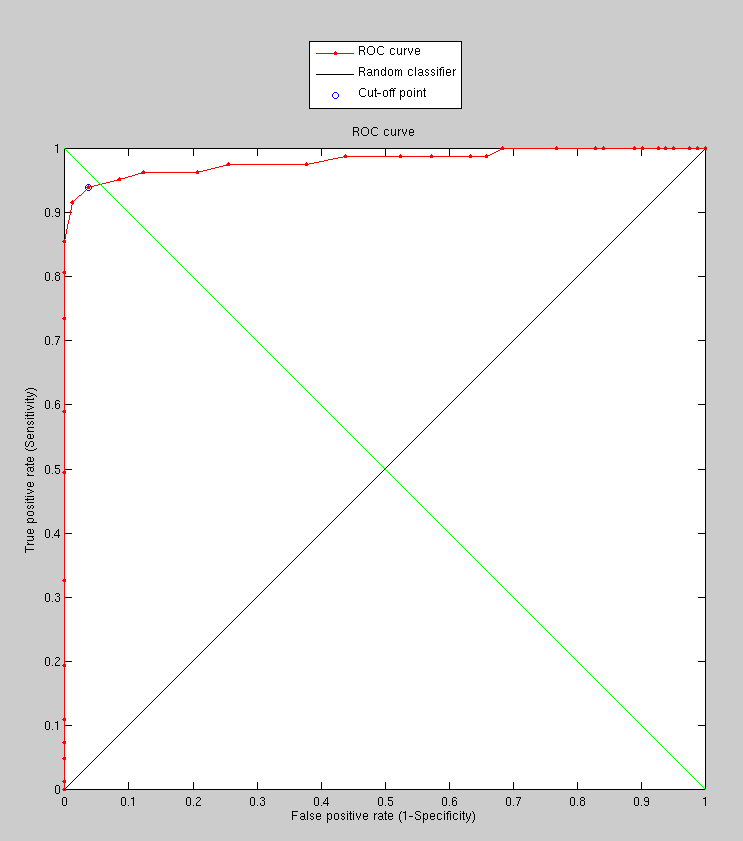
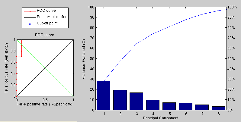
Using the same data and preprocessing as before (for the sake of a sound comparison), we have applied a PCA-based approach to get the following results, which are clearly by far superior. The variation incurred by expression is detected by PCA in the sense that it is not seen as a new type of variation.
|
The performance, as shown in Figure ![[*]](/IMG/latex/crossref.png) , is
therefore greatly improved and there is room for further improvements
as this implementation uses tiny images to save time and it does not
use the sophisticated approaches partly implemented by now. We need
to explore and compare breeds and variants of the same methodology,
which is easier to get to grips with when the matrices are of scale
that can be viewed and understood by a human (breakdown of the modes
of variation is shown at the top-right corner). Caveats can summarised
as follows:
, is
therefore greatly improved and there is room for further improvements
as this implementation uses tiny images to save time and it does not
use the sophisticated approaches partly implemented by now. We need
to explore and compare breeds and variants of the same methodology,
which is easier to get to grips with when the matrices are of scale
that can be viewed and understood by a human (breakdown of the modes
of variation is shown at the top-right corner). Caveats can summarised
as follows:
). To really improve performance
we must address the real caveats as well.
As a more novel experiment, we could use an approach for expression classification (possibly with the GIP dataset assigned for training).
|
We are still improving performance, despite all the caveats that remain
inherent. Improving performance by exploring different similarity
measure helped yield Figure
and Figure .
With the GIP data given us from the lab, it ought to be possible to
perform expression classification based on a set of expression models.
It should, in principle, be easy to build a model for each expression
and then test our ability to classify an unseen picture/3-D image
for the expression embodied and shown by it. In order to distinguish
our work from that of UWA (which I firmly believe took some shortcuts),
a classification benchmark17 would be worth pursuing. FRGC 2.0 data can be used for multi-person
validation of the approach, preceding other experiments in a publishable
paper. The face recognition problem seem to be a crowded space and
the EDM approach is good for automatically tackling expression variations,
via variation decomposition. Alternatively, performance on par with
whatever is in the literature can be pursued, only with the goal of
showing an EDM-based approach to be inferior to another. The image
from Figure shows handling of
unseen images by an expression model.
|
In general, once we get a good enough recognition rate (say within range of the Mian et al.) for the FRGC data, we'll have to introduce a more generalised way of compensating for expressions. One would say GMDS, but again, other G-PCA approaches are possible.
In its present state, with data mostly consisting expression variation, program performance depends overwhelmingly on the ability to recognise and eliminate/blur out/cancel the expressions contribution. Model description length can be used to determine how much of the variation is due to expression change. Empirically, so far there are signs that it is working, however there might be other explanations for it. With noses superimposed and faces generally facing the camera, ICP does not play a major role. It's all about the handling of expression changes. Suffice to say, by just detecting rigid areas one could calculate a lot of attributes that identify an individual. Then there is texture, which can further validate it although we do not use texture at all (so far).
It would be nice to draw a link between GMDS and G-PCA. In fact, there is a nice way to link the two theoretically.
There have been some relevant talks available for viewing recently (over the Internet). So far, PCA seems to be serving primarily as a similarity measure with respect to entire sets of observations, where a given image gets compared - via residuals - to a set of other images of its kind. Surely there exist better uses for PCA; in the context of this work it gets used as a throwaway tool for measuring similarity, which utilises little of the information conveyed in the learning process.
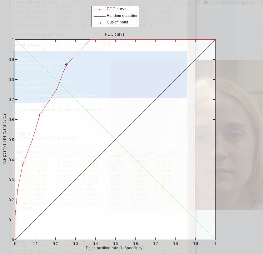
Manual markup of data or classification/pairing based on common properties (by hand) is extremely time consuming, especially if large sets become part of the protocol. In order to test on pairs excluded from the training process and then compare them to non-correspondent pairs (with or without expression), an experiment was designed to take 1,000 random pairs and compare them to: 1) unseen pairs with expression (figures below) pairs from similar sets of people (figures below). The results do show the ability to distinguish, but for more impressive results we will need to address existing caveats, which include the number of images building the mode and their size, among other important factors. It will take more time. The University of Houston did not respond to request for such data.
|
|
Addressing the caveats in turn, we can start compensating for set sizes by manually selecting more of them, then building models of a greater scale (high level of granularity). What would further complicate the process is an inclusion of a wide range of separate expressions, without separation between them. The next experiments will elevate the level of difficulty by basically modeling the variation within many existing pairs, first without special expressions and later with all sorts of unknown expressions. The goal then it to show detection rates with or without expressions, either in the training set or the partition of targets. Experiments will take longer to design (requires manual organisation per individual) and also to run. The favouring of arduous tasks helps distinguish between good methods from lesser effective ones, especially at edge cases. If run on simpler sets, the results will improve considerably.
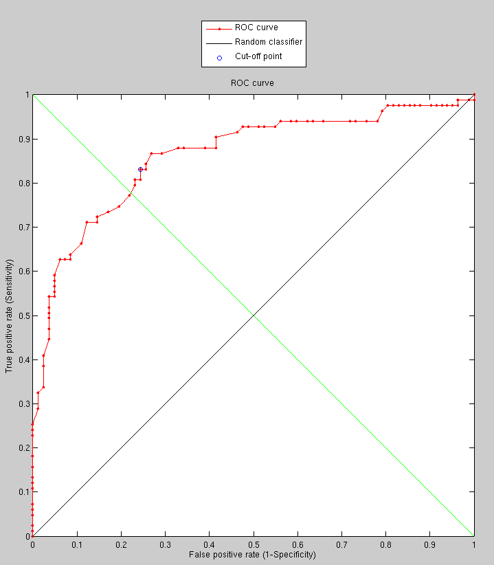
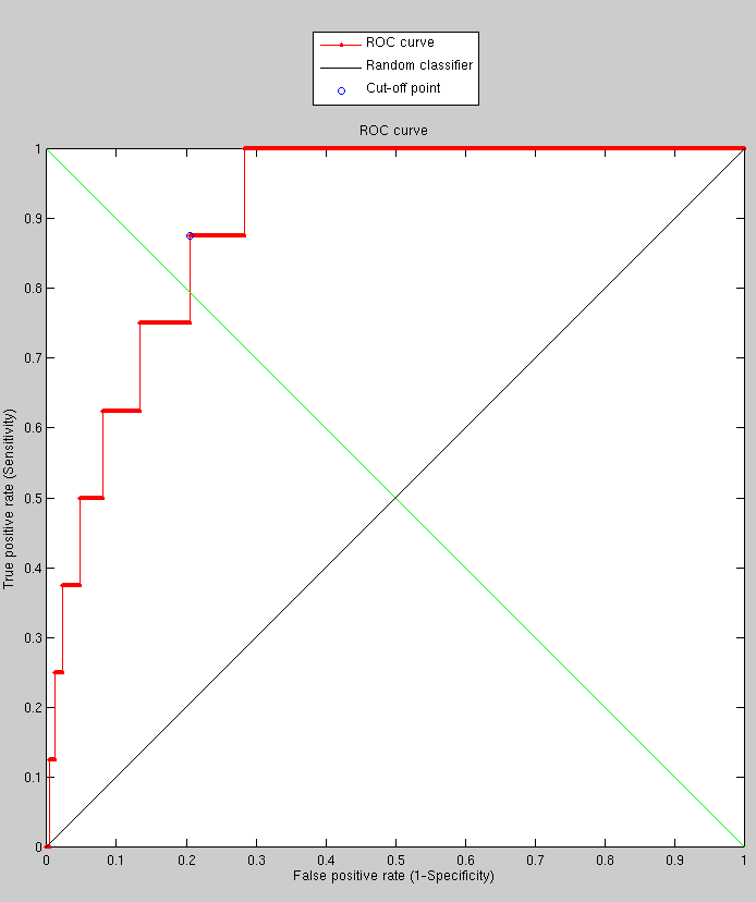
It has become evident that by doubling the sampling density, the models
are now a bit more detailed and they incorporate more pertinent bits
of information. To merely test the surface, the harder sets (from
the fall semester) had been taken and
10 individuals were selected from there. Using 100 images (i.e. 50
residuals) in total we build a model and we set aside images of the
same 10 individuals - those which will be containing 10 residues.
These are separate from the training set. Checking model match for
these 10 images and then comparing that with random pairs we get the
following ROC curve which Figure depicts.
|
Selected from the set to be used as correct pairs are just the first
10 people, do there is no cherry-picking. The random selection of
the rest is truly random, too. The reason for the nature of this experiment
is that it is extensible in the sense that we can carry on selecting
people sequentially from the set (a lot of manual work required) and
set the number of false pairs to be anything we like, as the random
selection leaves NxN possible pairing for the N![]() 4,000
images that we have at our disposal.
4,000
images that we have at our disposal.
The next step would involve introducing more images into the experiment. If that good use of time turns out to give equally promising results, then other experiments can be designed with similar images too.
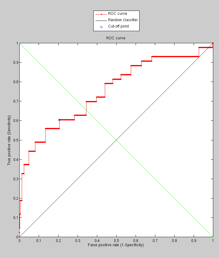
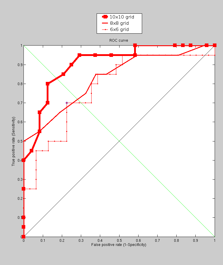
Granularity level, where sample point separation for PCA is 6x6, 8x8 and 10x10 (10 pixels/voxels apart), was next tested for better understanding of the space being explored, and subsequently for insight into how to set parameters. The next experiment explores the impact of granularity level in model-building on the overall performance. In order to make the experiments more defensible, the training set is changed from a size that can be described as minimalist (100 images) to 170, which requires further manual work. The model is being built from this set and performance then tested as before. The number of targets has been doubled. The experiments are still extensible in the sense that they can be rerun with a larger set.
The process involves building a model (limitations on the size of
the training set notwithstanding), then doing assessment work on the
target set with correct matches and another target set with incorrect
matches, repeating for each model granularity level. These experiments
take many hours to perform and so far it can be shown that by sampling
more and more points performance is actually degraded rather than
improved. This is not so counter-intuitive because by oversampling
we lose sight or focus of large-scale structures and start comparing
almost-to-be-treated-as-textural changes on the surface, including
teeth for example. This probably needs a more careful look for better
comprehension. Many of the caveats remains, particularly set sizes
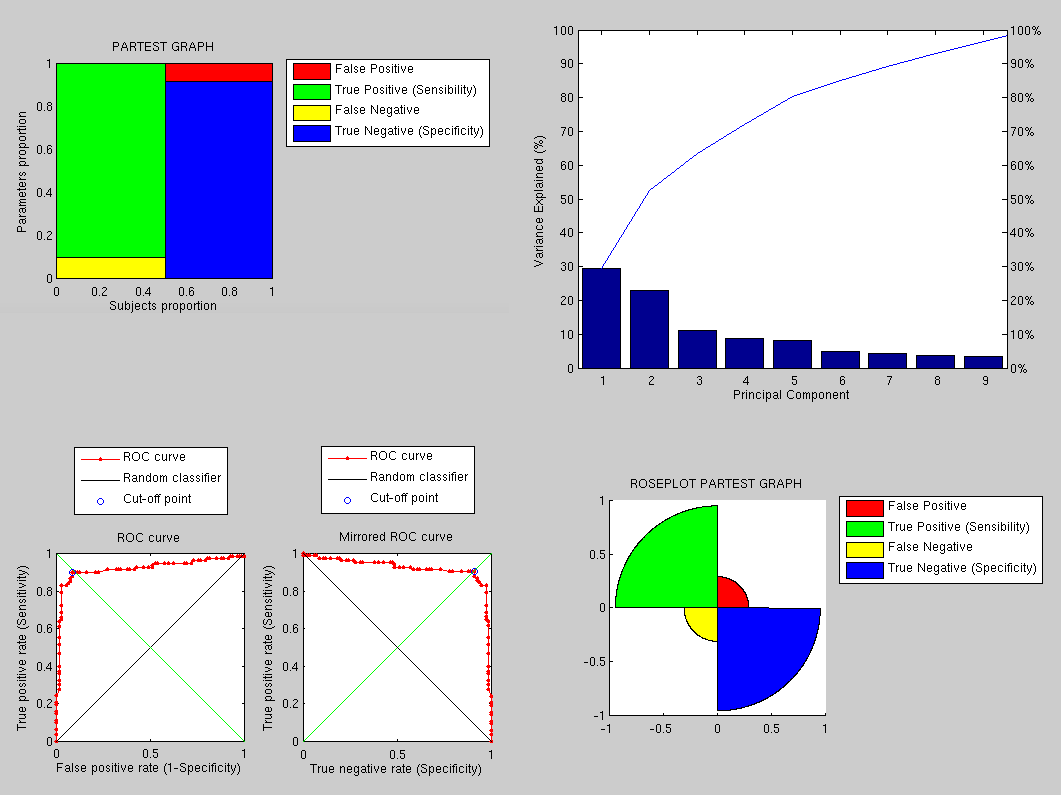
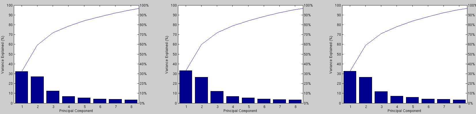
and the nature of chosen datasets. Figure
shows the results and Figure helps
validate the consistency among the cases.
|
|
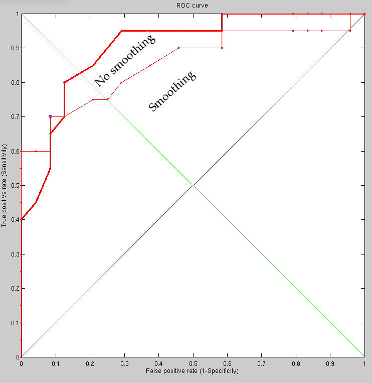
Smoothing was considered but hadn't been implemented as it was assumed that with enough points the impact would be limited. Points were knowingly sampled at fixed intervals without compensating for neighboring points in the vicinity/locality.
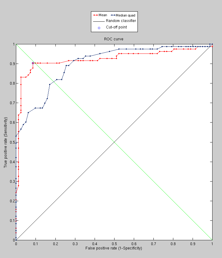
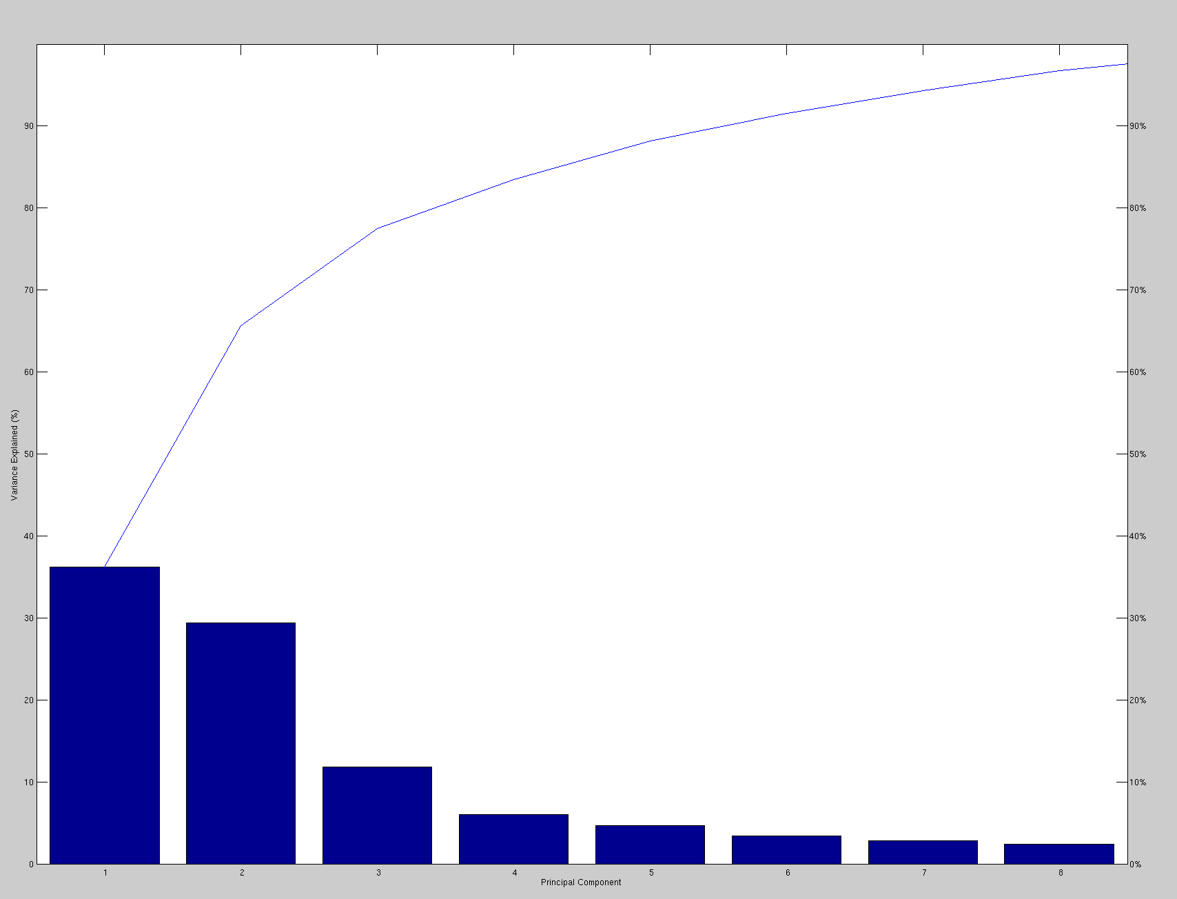
With smoothed surface sampling we get slightly different results,
based on a couple of experiments I ran; the results of the smaller
one are shown in the image. As the image in Figure
shows, if we smooth before sampling, then the results are actually
degraded (accompanying model decomposition in Figure ).
Maybe the smoothing was just excessive, or maybe the experiments were
not large enough to inspire confidence (the error bars would be large
if they were plotted). We could run the same experiments on unseen
faces with expressions in all pairs in order to get smoother ROC curves,
but it is really performance which needs to be addressed first (getting
into the ballpark of 90% recognition rate or better for difficult
sets/edge cases).
The next experiment explores a new model-based approach that I am implementing as the current approach leaves much to be desired and it also requires far bigger sets for training of the model. The group of people whom we are emulating used thousands of images for training and these images were not part of the FRGC set. Currently we use a poor training set which is also very small, so the models are of poor quality, just like the targets. Nevertheless, this enables ideas to be explored, at least in the proof of concept stage, and it generally works.
|
|
It is reasonable to assume the smoothing most probably occurred already at the scanner level, and additional smoothing may damage the information rather than just act as an anti-alias filter.
Roy Schestowitz 2012-01-08