 OR a little bit of background on tagging and my current work, see my previous posts on the subject [1, 2, 3], prior to me getting data from Professor Axel. The goal is to advance existing methods that include tagging by applying to them an algorithm which I developed for non-rigid registration assessment in the brain. This time the data that I deal with is cardiac, so temporal sets are a far more complicated problem, particularly due to persistent motion. Of interest there’s the paper “Single Heartbeat Cardiac Tagging for the Evaluation of Transient Phenomena” from Daniel A. Herzka, J. Andrew Derbyshire, Peter Kellman, and Elliot R. McVeigh. It can be found in Magnetic Resonance in Medicine (Volume 54, Issue 6, pages 1455–1464, December 2005) and the full paper says in its abstract: “Many cardiac abnormalities are of a transient nature, creating a beat-to-beat variation in myocardial function. This work presents the cardiac imaging technique for the measurement of regional function during transient cardiac phenomena. All information necessary for the reconstruction of a cine loop is acquired within a single heartbeat, avoiding the temporal blurring introduced by segmented imaging due to the assumption of cardiac cycle periodicity…”
I shall assume that motion can be treated like changes that occur over time on different dates or across subjects. The part in the above paper which deals with tags is: “Images reconstructed from such data displayed tag blurring and reduced tag persistence due to motion and interheartbeat variability. Images acquired during the Valsalva maneuver demonstrated apparent beat-to-beat variability, visible both in the images and as changing strain patterns and ventricular volumes.”
Therein lies a real problem because the tags cannot be assured to exist where they are needed the most. Fortunately, the literature contains many examples of work that can reconstruct imaged objects based on spatial information other than the tags themselves. A paper which was cited a lot in the 90s comes from Young and Axel (published in 1992, but date of current version is 6th of August 2002) and it is titled “Non-rigid heart wall motion using MR tagging”. Prior to it, in 1988, E A Zerhouni, D M Parish, W J Rogers, A Yang, and E P Shapiro looked at ways of analysing myocardial motion, potentially in troubled patients. Their paper “Human heart: tagging with MR imaging–a method for noninvasive assessment of myocardial motion” is summarised thusly:
Specified regions of the myocardium can be labeled in magnetic resonance (MR) imaging to serve as markers during contraction. The technique is based on locally perturbing the magnetization of the myocardium with selective radio-frequency (RF) saturation of multiple, thin tag planes during diastole followed by conventional, orthogonal-plane imaging during systole. The technique was implemented on a 0.38-T imager and tested on phantoms and volunteers. In humans, tags could be seen 60-450 msec after RF saturation, thus permitting sampling of the entire contractile phase of the cardiac cycle. Tagged regions appear as hypointense stripes, and their patterns of displacement reflect intervening cardiac motion. In addition to simple translation and rotation, complex motions such as cardiac twist can be demonstrated. The effects of RF pulse angle, relaxation times, and heart rate on depiction of the tagged region are discussed.
The German Heart Institute Berlin published the paper “Magnetic resonance stress tagging in ischemic heart disease” many years later (2005) and they used a 1.5-Tesla scanner for probing patients with coronary artery disease (CAD) under high-dose dobutamine stress. This clinical study helped show how “quantitative myocardial tagging may become a tool that reduces the need for high-dose dobutamine stress.”
As stated in previous posts and short papers which will be uploaded at a later date, my intention is to consider stress/strain analysis applied to the imaged tags. It is the tracking of the tags and making use of them that’s very challenging around boundaries that move throughout the cardiac cycle. Identifying templates like a cross where the tags have an intersection is a computationally expensive process that may also require taking uncertainty into account. If the goal is to track tags in real-time-level speeds (like in some ultrasound packages), then a faster approach is needed, e.g. shuffle distance. This approach would involve comparing different frames (at least one prior frame, with the exception of the first which has no predecessors) and then, in the junctions of the tags, best matches will be found and recorded in a vector of {x,y} coordinates, where these coordinates are refined over time and help quickly determine the motion of objects inside the image. Calculations using mechanical models (based upon shapes that the tags form) are an area which is already well explored, so it is the tracking and recovery of tags which my code deals with first and foremost. prototyping is done in GNU Octave, which helps make a visual proof of concept on arbitrary data, either synthetic or real. The code below does not yet do much, but once it’s finalised the code will be published properly.
Octave functions of relevance (still experimental and the GPLv3-licensed BioSig project may be required, as noted here):
function [new_image] = getdicomimages(directory, threshold)
% GETDICOMIMAGES: Open and test DICOM images of the heart
%
%    Licensing
%
%      GNU GPL version 3
%
%    GENERAL
%
%      Script - experimental, for handling MRI images with biosig
%
%    INPUT/S
%
%      -Omitted
%
%    OUTPUT/S
%
%      -Omitted
%
%    PENDING WORK
%
%      -
%
%    KNOWN BUG/S
%
%      -None.
%
%    COMMENT/S
%
%      -
%
%    RELATED FUNCTION/S
%
%
%
%    ABOUT
%
%      -Created:     November 2010
%      -Last update: November 5th, 2010
%      -Revision:    0.0.1
%      -Author:      Dr. R. S. Schestowitz
% ==============================================================

%// addpath ("/home/roy/Main/IT/Programs/get_dicom_heart")
%// addpath ("/home/roy/Main/IT/Programs/biosig4octmat-2.50/biosig/t200_FileAccess")
%// img = opendicom("~/Main/IT/Programs/MR-Cardiac/i148713.MRDC.1");  // deprecated function
%// sopen("~/Main/IT/Programs/MR-Cardiac/Full-CD/DICOM/ST000000/SE000019/MR000000");
%// img(i)=imread('sombrero.jpg')
%// plot(img.T0)   //metadata attributes
%// ~/Main/IT/Programs/dicom2/dicom2 ~/Main/IT/Programs/MR-Cardiac/Full-CD/DICOM/ST000000/SE000014/*

cd(directory);
files_list=ls('*.tga');
n_images=size(files_list,1);
% BIOSIG open function, wrapper to DICOM handler:
% img = sopen("~/Main/IT/Programs/MR-Cardiac/i148713.MRDC.1");
for i=1:1:n_images,
	% files_list
	%// img_metadata(i) = sopen(files_list(i,:))
	%a=imread(files_list(i,:));
	%imshow(a)
	figure;
	img(:,:,i)=imread(files_list(i,:));
	imshow(img(:,:,i))
end
For actual testing:
function [new_image] = loadtaggedsequence(directory, threshold, draw_grid)
% LOADTAGGEDSQUENCE: Open and test tagged images of the heart
%
%    Licensing
%
%      GNU GPL version 3
%
%    GENERAL
%
%      Script
%
%    INPUT/S
%
%      -Omitted
%
%    OUTPUT/S
%
%      -directory: location of images,
%	 -threshold: colour of tags/markers based on conrtast of image
%      -draw_grid: boolean for display of manual grid/points (drawing or not drawing)
%
%    PENDING WORK
%
%      -
%
%    KNOWN BUG/S
%
%      -None.
%
%    COMMENT/S
%
%      -
%
%    RELATED FUNCTION/S
%
%
%
%    ABOUT
%
%      -Created:     November 2010
%      -Last update: November 10th, 2010
%      -Revision:    0.0.1
%      -Author:      Dr. R. S. Schestowitz
% ==============================================================

% common commands

	%// loadtaggedsequence('~/Main/IT/Programs/MR-Cardiac/Zhen-thesis',1,1)
	%// addpath ("/home/roy/Main/IT/Programs/get_dicom_heart")
	%// addpath (genpath("/home/roy/Main/IT/Programs/biosig4octmat-2.50/biosig/"))
	%// path
	%// img = opendicom("~/Main/IT/Programs/MR-Cardiac/i148713.MRDC.1");  // deprecated function
	%// sopen("~/Main/IT/Programs/MR-Cardiac/Full-CD/DICOM/ST000000/SE000019/MR000000");
	%// img(i)=imread('sombrero.jpg')
	%// plot(img.T0)   //metadata attributes
	%// ~/Main/IT/Programs/dicom2/dicom2 ~/Main/IT/Programs/MR-Cardiac/Full-CD/DICOM/ST000000/SE000014/*

% experimental options

draw_circles=0;

% grid parameters

x_start = 10;
y_start = 10;
step_x = 30;
step_y = 20;
x_max = 110;
y_max = 80;


frame_size=8;
shuffle_radius=3;

% initialisation

first_image=1;
old_boundaries=[[0,0];[0,0]];

% get data

cd(directory);
files_list=ls('*.png');
	% files_list=ls('*.gif');
	% One image: files_list=('seq-tag-1.png');

% Opening [print filenames if necessary]

files_list
n_images=size(files_list,1);

% main loop

	% img = sopen("~/Main/IT/Programs/MR-Cardiac/i148713.MRDC.1");
for i=1:1:n_images,
		%// img_metadata(i) = sopen(files_list(i,:))
		%a=imread(files_list(i,:));
		%imshow(a)
	figure;
	%img(:,:,i)=imread(files_list(i,:));

	if (draw_grid==1)
		for j=x_start:step_x:x_max,
	   	  img(j,:,i)=0;
		end
		for j=y_start:step_y:y_max,
	   	  img(:,j,i)=0;
		end
	end
	if (draw_circles==1)
	     % [center,radius]=sphfit([10,11,0],[5,5,0]);
        end
	boundaries=[[x_start,y_start];[x_start,y_start+step_y]; ...
	[x_start,y_start+step_y*2]; [x_start,y_start]; ...
	[x_start+step_x,y_start];[x_start+step_x*2,y_start]; ...
	[x_start+step_x*2,y_start+step_y];[x_start+step_x*2,y_start+step_y*2]; ...
	[x_start+step_x,y_start+step_y];[x_start+step_x,y_start+step_y*2]];
	%%	boundaries_x=[;    %% deprecated - no more xy separation
        	for l=1:1:size(boundaries,1)
        	%%	for k=1:1:size(boundaries,2)
        		% debugging
        		%	boundaries_y(k,1);
        		%	boundaries_y(2,l);
                     	% img(1,3,1)=1;
                     	% boundaries_y(k,1)
                     	% boundaries_y(2,l)
                     	%i
                     	%k
                     	%l
                     	% size(boundaries_y,1)
                     		if (first_image==0)
                     			%old_boundaries
                     	    		new_dot_x=old_boundaries(l,1)+1;
                     	    		new_dot_y=old_boundaries(l,2)+1;
                     	    			%old_boundaries(l,1)-8
                     	    		search_frame_current=img(((new_dot_x-frame_size):(new_dot_x+frame_size)),((new_dot_y-frame_size):(new_dot_y+frame_size)))
                     	    		search_frame_previous=img(((old_boundaries(l,1)-frame_size):(old_boundaries(l,1)+frame_size)),((old_boundaries(l,2)-frame_size):(old_boundaries(l,2)+frame_size)))
                     	    		shuffle_diff=shuffle_transform(search_frame_current, search_frame_previous, shuffle_radius)

                     	    		img(new_dot_x,new_dot_y,i)=threshold/255;
                     	    		old_boundaries(l,1)=new_dot_x;
                     	    		old_boundaries(l,2)=new_dot_y;
                     		else
                     	    		img(boundaries(l,1),boundaries(l,2),i)=(255-threshold)/255;
                     		end
                    %% 	end
        	end
        	%for l=1:1:size(boundaries_x,1)
        		%for k=1:1:size(boundaries_x,2)
                     	   %img(boundaries_x(k,2),boundaries_x(l,1),i)=250;
                	%end
        	%end
	imshow(img(:,:,i))
		% plot3(img(:,:,i))
        if (first_image==1)
	   old_boundaries=boundaries;
	end
        first_image=0;
end
Peripheral transform:
function [value,shuffle] = shuffle_transform(image,im2,radius)
% SHUFFLE_TRANSFORM: A shuffle transform based on an implementation by Steve Marsland
%
%    Licensing
%
%      -
%
%    GENERAL
%
%      Function
%
%    INPUT/S
%
%      -image: first image
%      -im2: second image
%      -radius: the shuffle radius
%
%    OUTPUT/S
%
%      -Omitted
%
%    PENDING WORK
%
%      -
%
%    KNOWN BUG/S
%
%      -None.
%
%    COMMENT/S
%
%      -
%
%    RELATED FUNCTION/S
%
%
%
%    ABOUT
%
%      -Created:     November 2010
%      -Last update: November 21st, 2010
%      -Revision:    0.0.1
%      -Author:      Dr. R. S. Schestowitz
% ==============================================================

shuffle = zeros(size(image));

for i=radius+1:size(image,1)-radius
    for j=radius+1:size(image,2)-radius
        template = im2(i-radius:i+radius,j-radius:j+radius);
        diff = abs(template-image(i,j));
        shuffle(i,j) = min(diff(:));
    end
end
value = mean(shuffle(:))

 HIS is the second part of a discussion about ways in which GNU/Linux adoption is being discouraged, with or without Microsoft’s direct involvement. Gordon, Tim, and Roy speaks about no article in particular this weekend; instead they concentrate on many examples from the past few years. Tim’s site, OpenBytes, will publish some some show notes very shortly. We made no preparations for the shows, so notes are put together only after the discussion.
![]() Today’s show ends with “SPARKLE” by Honey Sac (published in SXSW 2009 Showcasing Artists). Marti is working on a new intro for the show and we also hope to have him — as well folks from Mageia — on an imminent episode. We hope you will join us for future shows and spread the word if you enjoy this show. Also consider subscribing to the show via the RSS feed. If you have an Identi.ca account, consider subscribing to TechBytes in order to keep up to date.
Today’s show ends with “SPARKLE” by Honey Sac (published in SXSW 2009 Showcasing Artists). Marti is working on a new intro for the show and we also hope to have him — as well folks from Mageia — on an imminent episode. We hope you will join us for future shows and spread the word if you enjoy this show. Also consider subscribing to the show via the RSS feed. If you have an Identi.ca account, consider subscribing to TechBytes in order to keep up to date. 


 Filed under:


 OR a little bit of background on tagging and my current work, see my previous posts on the subject [
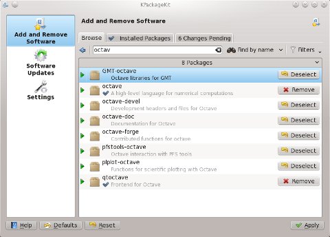
 ‘ve been an Octave user on several machines and everything worked perfectly well until Fedora 14, which has a newer version of the software and thus a serious conflict of incompatible libraries. For many image loaders the following type of error is shown just before Octave crashes: