few years ago the DARPA Grand Challenge explored that scarcely understood potential of autonomous vehicle navigation with on-board, non-remote computer/s and a fixed number of viewpoints (upper bound on apertures, processing power, et cetera). This received a great deal of press coverage owing to public interest, commercial appeal, and the general underlying novelty. While the outcome was promising, not many people are able to afford the equipment at hand. With mobile devices proliferating, semi-autonomous or computer-aided driving becomes an appealing option, just as surgeries are increasingly involving assistance from computers (c/f MICCAI as a conference). This trend continues as confidence in the available systems increases and their practical use is already explored in particular hospitals where human life is at stake.

Road regulations currently limit the level to which computers are able to control vehicles, but in the US those regulations are subjected to constant lobbying. Many devices utilise GPS-obtained coordinates, but very few exploit computer vision methods to recognise obstacles that are observed natively rather than derived from a map (top-down). A comprehensive search around the Android repository reveals very little work on computer vision among popular applications. Processor limitations, complexity, and lack of consistency (e.g. among screen sizes and camera resolution) pose challenges, but that oughtn’t excuse this computer vision ‘drought’. A lot of code can be conveniently ported to Dalvik.

In order to explore the space of existing work and products, with special emphasis on mobile applications, I have begun looking at what’s available for navigation bar stereovision (as it would require multiple phones or a detached extra camera for good enough triangulation). Tablets and phones make built-in cameras more ubiquitous, alas their full potential is rarely realised, e.g. when docked upon a panel in a car with a high-resolution, high capture rate (framerate) camera.

According to Wikipedia, “Mobileye is a technology company that focuses on the development of vision-based Advanced Driver Assistance Systems” and this system is geared towards providing the user with car navigation capabilities that are autonomous and rely only on a single camera, such as the one many phones have. Functionality is said to include Vehicle Detection, Forward Collision Warning, Headway Monitoring & Warning, Lane Departure Warning and Lane Keeping / Lane Guidance, NHTSA LDW and FCW, Pedestrian Detection, Traffic Sign Recognition, and Intelligent Headlight Control. The company received over $100 million in investment as the computer-guided navigation market seems to be growing rapidly. A smartphone application is made available by Mobileye, with a demo version available for Android. “Although the Mobileye IHC icon will appear on the application, it requires additional hardware during installation,” their Web site says. The reviews by users are largely positively (demo version, 1.0, updated and release January 5^th, 2012).

The collective of Android apps for car navigation suggests that it’s a crowded space, but a lot uses GPS and not computer vision.

The video “Motorola Droid Car Mount Video Camera Test” shows the sort of sequence which needs to be dealt with. Lacking hardware acceleration it would be hard to process frames fast enough (maybe the difference between them would be more easily manageable). Response time for driving must avert lag. It’s the same with voice recognition on phones as it’s rarely satisfactory in real-time mode. Galaxy II, for example, takes a couple of seconds to process a couple of words despite having some very cutting-edge hardware.

We (myself and colleagues, especially myself) are unable to get good performance by edge detection and other ordinary means, especially because in 3-D things are more fuzzy. We will try normals again in the coming days.

I have been trying long and hard to vary parameters and tinker with what’s available in the image in order to place points at edges and corners, but the performance is never better than when ICP is used to put the points at the same location on the grid (after alignment by ICP of course).

Image 1:

Image 2:

I have been working to compare and assess how using inner circles/rings would improve our older implementation which mostly judges similarity based on outer circles/rings. This test can be improved a lot by choosing more points, but it will take time to get the results.

Image 3:

Image 4:

Departing back to older methods which use one single criterion for verification and also use coarse sampling of the surface, performance is not encouraging; but the next step will to be an attempt to use surface normals or another bit of information which can be derived from the surface alone.

Image 1: Results of a coarse approach tested on ~400 pairs.

Image 2: Example of a pair of images.

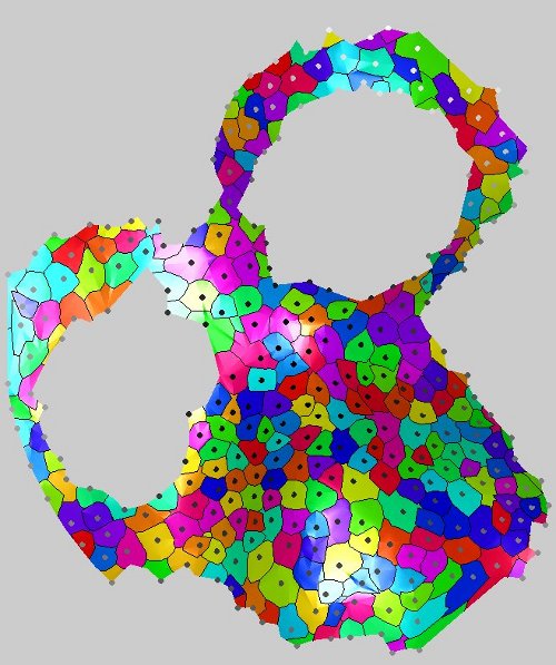
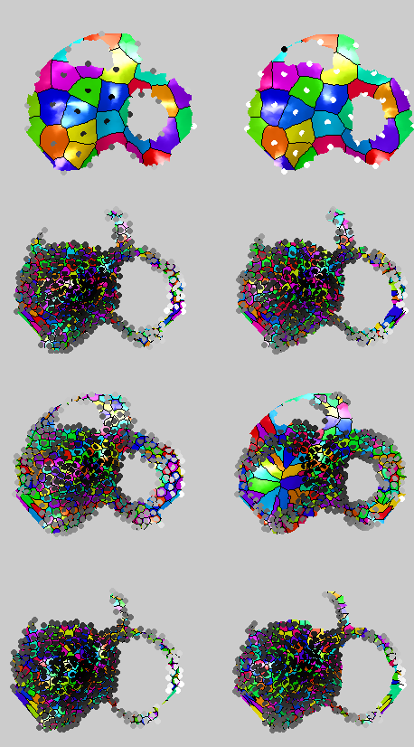
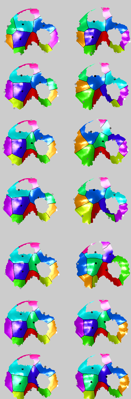
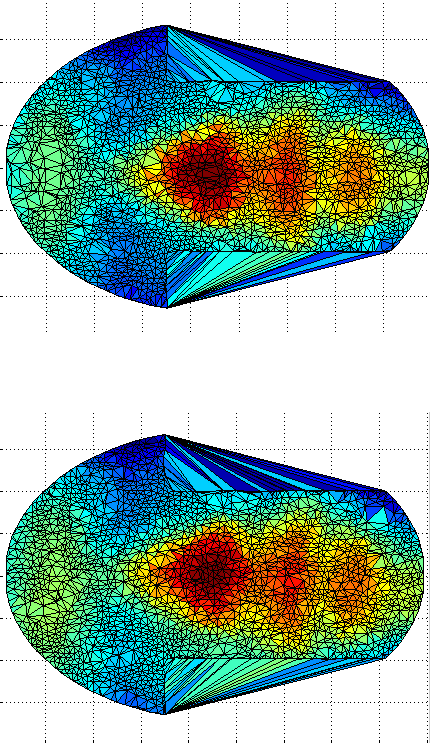
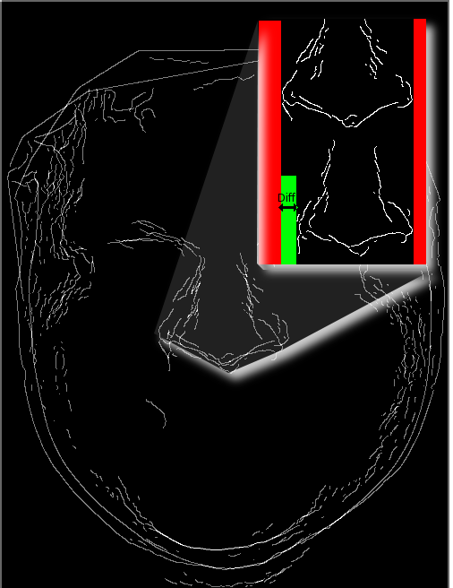
N OUR pursuit of a similarity measure for anatomical surfaces (biomedical or otherwise external to one’s body), integration over the dot product between the normals is considered. This is a powerful correlation measure between aligned surfaces, i.e. integral |<normal_1,normal_2>| delta area. The higher the integral, the higher the correlation.

If we have the two surfaces given as S(x,y) and Q(x,y) and da(S) = \sqrt{S_x^2+S_y^2+1} and the normal is given by N_S(x,y) = {-S_x,-S_y,1}/da(S), then one option is: <N_S,N_q> da = (S_x*Q_x+S_y*Q_y+1)/da(Q). A more unbiased one is to integrate over: |S_x*Q_x+S_y*Q_y+1|(1/da(Q)+1/da(S)) after alignment.

Normals were explored for a while as the normals can truly be taken into account for measuring correlation between images. Here is what some noisy normals look like when scattered arbitrarily.

Normals should be better than surface area, but one should be careful with normals at the boundary, one should probably ignore them.

Surface Normals were tested for almost a week. On its own, the integral produces a similarity measure not superior to some that we already have, but it can be used to further improve classification, based on another distinct method. Fixing the ranges for the integration is the trickier bit which needs more adjustment. I have been testing some variants around this measure, but there is still lots more that can be done (this ROC curve is based on a measure applied to entire images).

If we do not eliminate outlier noise first, there would be not much use to most l2-based measures.

Apropos, this new paper [PDF] came out which suggests one other way of using geodesic distances, more robustly. In order to take better advantage of spatial properties such as surface edges (greater steepness) and alignment among normals, the placement of points for geodesic methods has become based on such properties rather than having them spread randomly or at fixed positions as before. Results will be presented in a moment.

In the case of faces, slight occlusion is a real problem for us, e.g. around the nose/nostrils, not to mention hole filling around areas like the eyes. It weakens the measures. Real geodesics or workarounds can help mitigate the inaccuracy caused by this, but really, there is lack of information in particular parts and it’s inherently a problem. By dividing the image into partitions one can get more ‘localised’ distances, still based on graph theory and the Sethian et al. approach. The results in the paper are given for 2-D+3-D and are not quite so competitive; they are tested on databases I have not come across in the literature before. To measure geodesics around anatomically analogous points (not overlapping points after ICP), I am now using edges and normals; the hard part is adjusting thresholds such that across people the same points (e.g. nose edges) can be consistently detected.

Sobel on same person:

Roberts on same person:

Canny (edge detection algorithm) on same person:

Canny applied to different persons:

Using 3-D data alone, we wish to choose anchor points for FMM which are not determined exclusively by ICP (e.g. overlapping points after alignment). I have spent several days trying to use edge detection and normals to identify points around which to extend geodesic rings. So far, the results have not been encouraging enough; in fact, they’re less promising than while relying on ICP alone. Even the placements of overlapping points at random gave much better verification results.

Canny on same person:

Canny applied to different persons (subset shown as Voronoi cells):

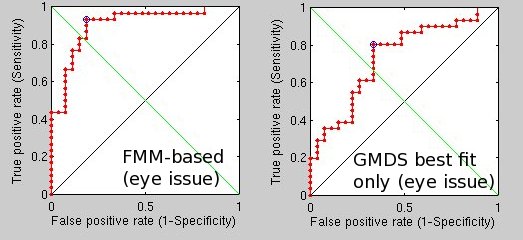
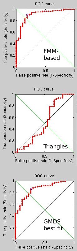
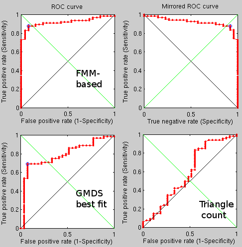
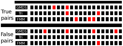
sing a more brute force approach which takes into account a broader stochastic process, performance seems to have improved to the point where for 50 pairs (100 images) there are just 2 mistakes using the FMM-based approach and 1 using the triangles counting approach. This seems to have some real potential, even though it is slow for the time being (partly because 4 methods are being tested at the same time, including two GMDS-based approaches).

I then restarted the experiment with 4 times more points, 84 images, and I’ll run it for longer. At the start there were no mistakes, but it’s slow. The purpose of this long experiment to see if length of exploration and use of numerous methods at once can yield a better comparator. In the following diagram, red indicates wrong classification. Since similarity is measured in 3 different ways, there is room for classification based on a majority, in which case only one mistake is made. It’s the 9th comparison of the true pairs, which is shown as well. The mouth and arguably whole lower part of the face is a bit twisted; the FMM-based approach got it right, but the other two failed. Previously, when the process was faster, the results were actually better.

Scatter alternations were made to investigate the potential of yet more brute force. I reran the experiments as before but with different parameters that scatter the random sample closer to the centre of the face and this eliminated the one mistake made before (9th true pairs). The changes resulted in one single result which was not correct: the 15th image in the other gallery. Whereas it was previously intuitive to find a fix for one mistake. when this fix introduces a mistake elsewhere it’s time to think of an approach change. One solution might be to increase the scatter sample/range, but it is already very slow as it is.

Edge detection was then explored as another classifier facilitator.

In order to address the recurring issue where misclassifications are caused by improper account for details versus topology, another approach is going to be implemented and added to the stack of methods already in use. The approach will use edge detection near anatomically distinct features and then perform measurements based on the output. As the image below shows, GMDS is still inclined to accept false pairs as though they are matching sometimes and this weakens the GMDS “best fit” approach.

I have implemented a 3-D classification method based on filters and Canny edge detector, essentially measuring distances on the surface — distances between edges. So far, based on 20 or so comparisons, there are no errors. But ultimately, this can be used as one classifier among several.

The thing is about Canny is, if we do that, we might as try using the set

Laplacian(I) - g(I)*div(g(I)/|g(I)|) = 0

where g(I) = grad (I) which is the Haralick part of the “Canny” edge detector, i.e. without the hysteresis integration.

I decided to look into changing it. Currently I use:

    % Magic numbers
    PercentOfPixelsNotEdges = .7; % Used for selecting thresholds
    ThresholdRatio = .4;          % Low thresh is this fraction of the high.
    
    % Calculate gradients using a derivative of Gaussian filter 
    [dx, dy] = smoothGradient(a, sigma);
    
    % Calculate Magnitude of Gradient
    magGrad = hypot(dx, dy);
    
    % Normalize for threshold selection
    magmax = max(magGrad(:));
    if magmax > 0
        magGrad = magGrad / magmax;
    end
    
    % Determine Hysteresis Thresholds
    [lowThresh, highThresh] = selectThresholds(thresh, magGrad, PercentOfPixelsNotEdges, ThresholdRatio, mfilename);
    
    % Perform Non-Maximum Suppression Thining and Hysteresis Thresholding of Edge
    % Strength
    e = thinAndThreshold(e, dx, dy, magGrad, lowThresh, highThresh);
    thresh = [lowThresh highThresh];

There is a lot that we can do with edges to complement the FMM-based classifiers (triangles count, GMDS, others), but moreover, I am thinking of placing markers on edges/corners (derived from range images) and then calculating geodesics between those. Right now it is all Euclidean, without account for spatial properties like curves in the vicinity. By choosing many points and repeating the process everything slows down, but previous experiments show this to bear potential. None of it is multi-scale just yet.

What we do with the edges is also risky, as the edges strongly depend on the pose estimation and expression. In pose-corrected pairs (post-ICP) I measure distances between face edges and nose edges. Other parts are too blurry and don’t give sharp enough an edge which is also resistant to expression. The nose is also surrounded by a rigid surface (pose-agnostic for the most part).

Problematic cases still exist nonetheless and I am trying to find ways to get past them. There are clearly problematic cases, such as this first occurrence in the 25th pair, where edge detection is not being consistent enough to make these distances unambiguous. In such cases, Euclidean measures — just like their geodesic counterparts — are likely to fail, incorrectly claiming the noses to be of different people.

A modified edge detection-based mechanism is now in place so as to serve as another classifier. It does fail as a classifier when edge detection fails, as shown in the image.

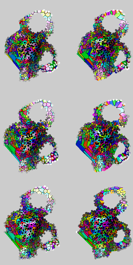
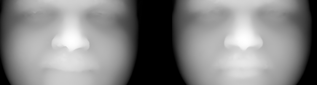
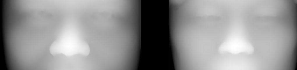
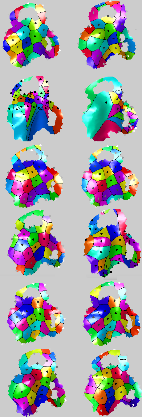
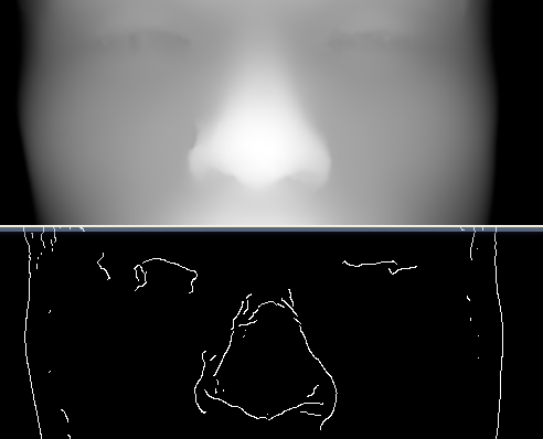
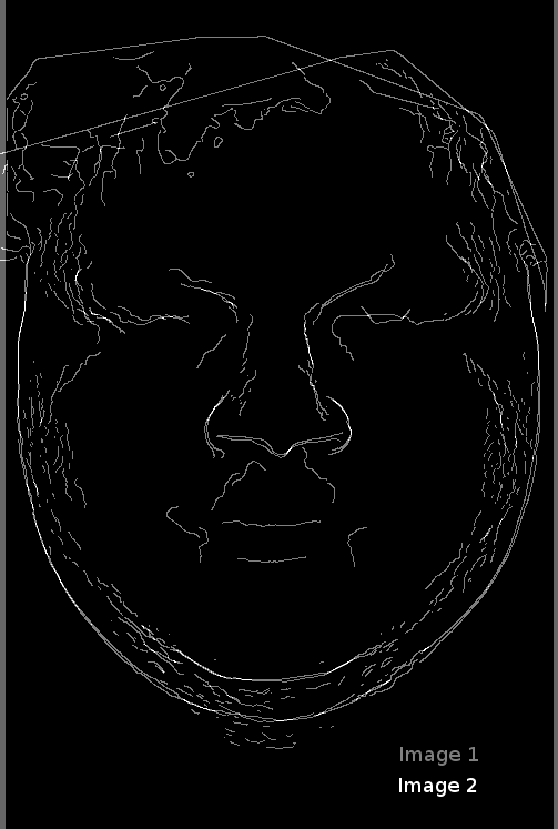
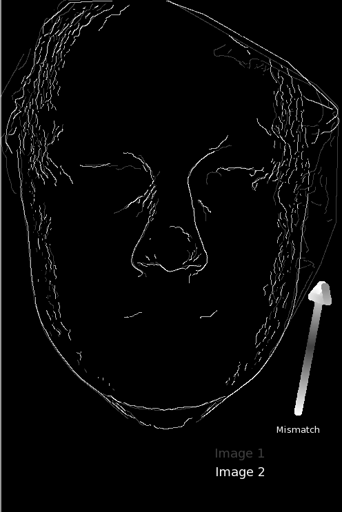
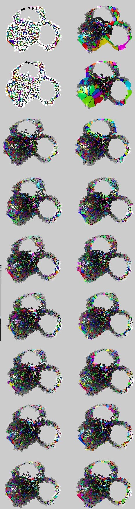
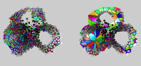
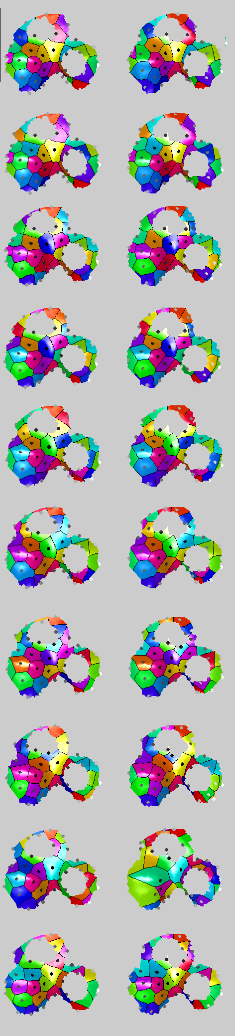
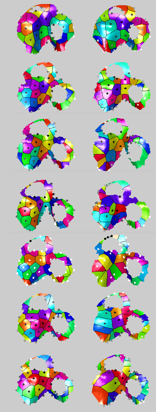
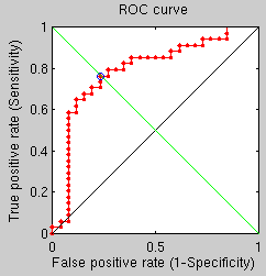
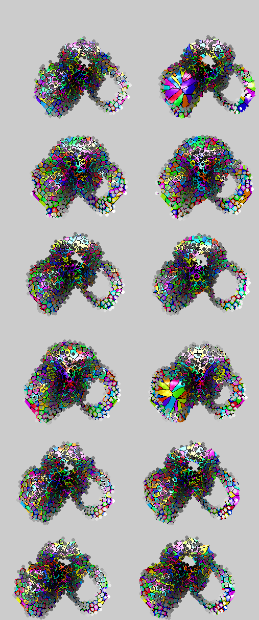
he latest batch of experiments looked at how one might cope with a mask closer than usual to the eye’s centre. I used harder pairs.

It did not work too well. One remaining limitation is that in an attempt to determine fiducial-esque points based on unmarked (not annotated) 3-D data there is little other than the nose tip that can consistently and accurately be pinned down. The eyes in particular are not simple to segment in 3-D — not without some help from 2-D anyway — mostly because the corners are fuzzy in 3-D. While slight head rotations can be annulled with ICP, there is still a difficulty associated with true distances as measured based on the range images. Accurately-measured geodesic distances are supposed to be robust to that, but in practice when there is slight rotation difference some of the calculations don’t add up. The sensitivity to inherent differences is often outweighed by pose.

Classification mistakes were partly caused by hair, occlusion, and other factors. I have rerun the same experiments as before with twice the number of vertices, but unsurprisingly, the results were about the same. The excessive detail gains never brought much improvement in terms of verification performance. Next, I took the best approach of the bunch and ran it on some of the hardest cases. The ROC curve is shown while for simpler cases the experiment is still being run on two servers.

There’s still no hope of beating state-of-the-art performance levels, unless of course a significantly improved variant is found.

Some of the problems are easier for the human eye to see, such as cases where hair penalises the scoring mechanism, as shown in the picture below.

Random points were then attempted, adding a stochastic nature to this problem. In order to make GMDS ‘fail’ most badly only in the case of false pairs, I have tested some new masks and measured verification performance reached by using them. For GMDS it failed quite badly, but with the other FMM-based approach — applied to some hard cases — I got the results shown in the ROC curve. Rather than dilating the masks and varying the hole sizes I would like to try varying positions from which to dilate in order to sample more distinct regions and measure distances upon those. This seems like an approach with real potential, provided the random (or fixed) sample of points is large enough to compensate for noise/intra-person variation. The latest experiment was preparatory towards this approach.

Random positions were further tested by making a variation, an improvement to the above. By letting the anchor points move around a bit (randomly within range) I was unable to get better performance than before (just over 90% verification rate on hard cases too). There are other methods that I could try next…

120 random positions were then placed on pairs to further test the approach. These further attempts to improve performance by moving points randomly (and this time taking a larger random sample) were not quite so successful. The general premise was, by taking many points around the face and expanding from them (with geodesic means) will lead to a good and rather unique signature. In practice, however, the measure is insensitive to real anatomical differences. Intra-person differences can outweigh inter-person differences. I’ll try another approach, but it will take days for results to arrive.

Although this is being tested on faces at the moment, the methods are generalisable and can be applied to any biomedical data for similar purposes.

n particular cases, GMDS failures (topological mistakes) continue to be a problem, but it is possible to detect whether that happens and then just filter those cases away. Having run experiments that try to overcome these occasional failures, I got nearly flawless classification with the FMM-based methods when it’s applied to simpler pairs, less successful when dealing with harder cases (an order of magnitude more failures, as shown in the ROC curve).

In order to reduce the recurrence of failures I am varying the size of the holes and the overall surface area, noting that still, even for corresponding surfaces, there are sometimes cases of GMDS failure.

More ROC curves were learned thereafter. Dealing yet again with cases that are hard, the following results were obtained by making further changes to the masks, even though ongoing experiments look at a wider range of attempts, over which a best fit or average get taken. By mixing the more successful approaches, better rates can be assured. By adding the simpler pairs, better rates can also be assured.

fter persistence and a new type of mask put in place (with a little trick to penalise for miscorrespondence around the top) I have been getting good validation results again, with over 98% for the first 50 pairs I have tested (just one mistake some far). Some of the harder surface pairs have not been reached yet.

In an attempt to master GMDS as cross-identity discriminator I have further cut down the process, which now operates through a pipeline of reverse dilation, as shown in the first image beneath. The second shows a broader mask working upon false pairs and mostly failing, which is probably what we want. In terms of performance, as long as the true pairs are similar enough (some are far harder than others, e.g. expression variation), we are able to get decent results. Running this on the whole database again would not help beat results that we got around December, though. Several experimental modifications are hard to identify as means of reverting back to old versions. A lot of those were made to facilitate diffusion as a supported (surrogate) option.

I have reduced the number of points in GMDS to just 10 because it seemed as though it would significantly speed up the process without compromising too much in terms of performance. The experiments were then run on “hard” pairs, giving verification performance of almost 90%, depending on the method used.

In an attempt to understand how well one can do with just 10 samples in GMDS (because it is faster and insensitive to small changes) I took some of the hardest classification cases and ran repeated coarse GMDS on them, reaching a success rate of only 75% or thereabouts. This falls short because we are assuming that only for false pairs will we have improper correspondence, whereas for true pairs everything will be perfect. As shown in the images produced from the same false pair, sometimes a good correspondence is found, but usually not (symbolised by white colours in the dots, e.g. in the third example from the top, on the right hand side).

The example at the very bottom shows that even for different identities a decent correspondence can be found, which gives rather low stress values.

In order to mitigate or altogether annul the effect/artifact of flipping, I have made the two surfaces asymmetric, with centres of the eyes removed because there’s too much noise there, depending where the eyes look and how open they are (in some surfaces, the eyes are deliberately moved to challenge algorithms).

Several empirical results show that increasing the number of vertices, even doubling them, still seems not to help much in any way. So, I have isolated some difficult cases and I am trying to cut out the sources of ambiguity.